Off-axis electron holography
LiberTEM has implementations for both hologram simulation and hologram reconstruction for off-axis electron holography.
New in version 0.3.0.
Hologram simulation
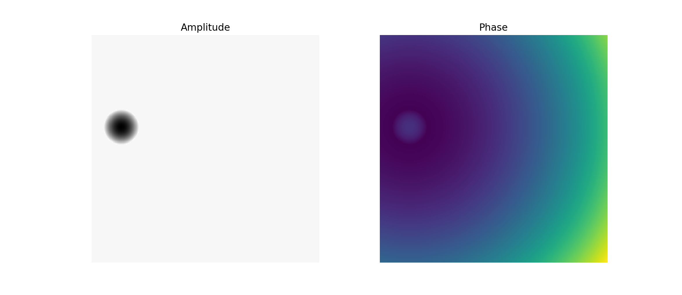
Holograms can be simulated using the method described by Lichte et al. [LL08] The simulator includes simulation of holograms with Gaussian and Poisson noise, without effect of Fresnel fringes of the biprism. The simulator requires amplitude and phase images being provided. Those can be calculated as in example below in which for amplitude a sphere is assumed, the same sphere is used for the mean inner potential (MIP) contribution to the phase and in addition to the quadratic long-range phase shift originating from the centre of the sphere:
import numpy as np
import matplotlib.pyplot as plt
from libertem.utils.generate import hologram_frame

# Define grid
sx, sy = (256, 256)
mx, my = np.meshgrid(np.arange(sx), np.arange(sy))
# Define sphere region
sphere = (mx - 33.)**2 + (my - 103.)**2 < 20.**2
# Calculate long-range contribution to the phase
phase = ((mx - 33.)**2 + (my - 103.)**2) / sx / 40.
# Add mean inner potential contribution to the phase
phase[sphere] += (-((mx[sphere] - 33.)**2 \
                   + (my[sphere] - 103.)**2) / sx / 3 + 0.5) * 2.
# Calculate amplitude of the phase
amp = np.ones_like(phase)
amp[sphere] = ((mx[sphere] - 33.)**2 \
               + (my[sphere] - 103.)**2) / sx / 3 + 0.5

# Plot
f, ax = plt.subplots(1, 2)
ax[0].imshow(amp, cmap='gray')
ax[0].title.set_text('Amplitude')
ax[0].set_axis_off()
ax[1].imshow(phase, cmap='viridis')
ax[1].title.set_text('Phase')
ax[1].set_axis_off()
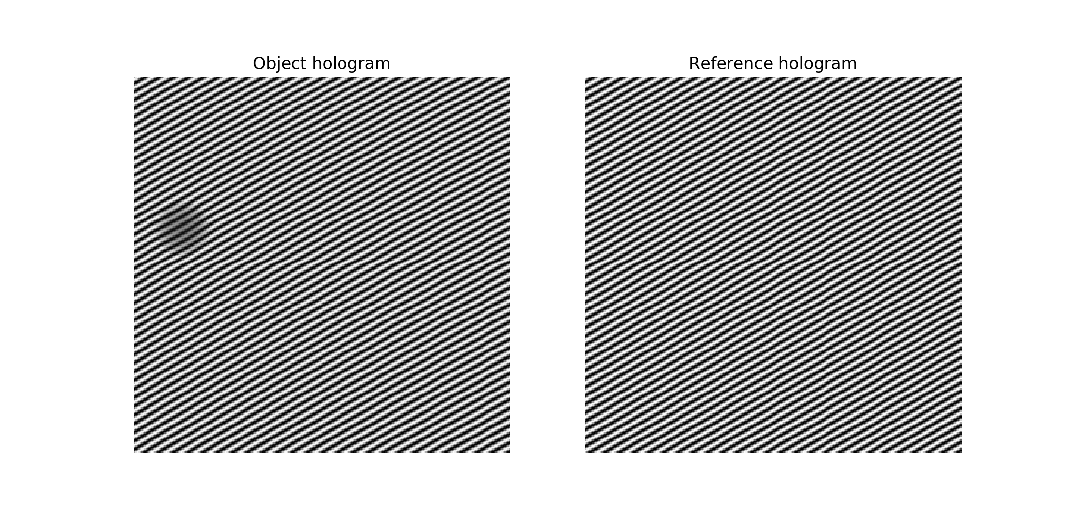
To generate the object hologram, amp and phase should be passed to the holo_frame
function as follows:
holo = hologram_frame(amp, phase)
To generate the vacuum reference hologram, use an array of ones for amplitude and zero for phase:
ref = hologram_frame(np.ones_like(phase), np.zeros_like(phase))

# Plot
f, ax = plt.subplots(1, 2)
ax[0].imshow(holo, cmap='gray')
ax[0].title.set_text('Object hologram')
ax[0].set_axis_off()
ax[1].imshow(ref, cmap='gray')
ax[1].title.set_text('Reference hologram')
ax[1].set_axis_off()
Hologram reconstruction
LiberTEM can be used to reconstruct off-axis electron holograms using the Fourier space method. The processing involves the following steps:
Fast Fourier transform
Filtering of the sideband in Fourier space and cropping (if applicable)
Centering of the sideband
Inverse Fourier transform.
The reconstruction can be accessed through the HoloReconstructUDF class.
To demonstrate the reconstruction capability, two datasets can be created from the holograms
simulated above as follows:
from libertem.io.dataset.memory import MemoryDataSet
from libertem.udf.holography import HoloReconstructUDF

dataset_holo = MemoryDataSet(data=holo.reshape((1, sx, sy)),
                             tileshape=(1, sx, sy),
                             num_partitions=1, sig_dims=2)
dataset_ref = MemoryDataSet(data=ref.reshape((1, sx, sy)),
                            tileshape=(1, sx, sy),
                            num_partitions=1, sig_dims=2)
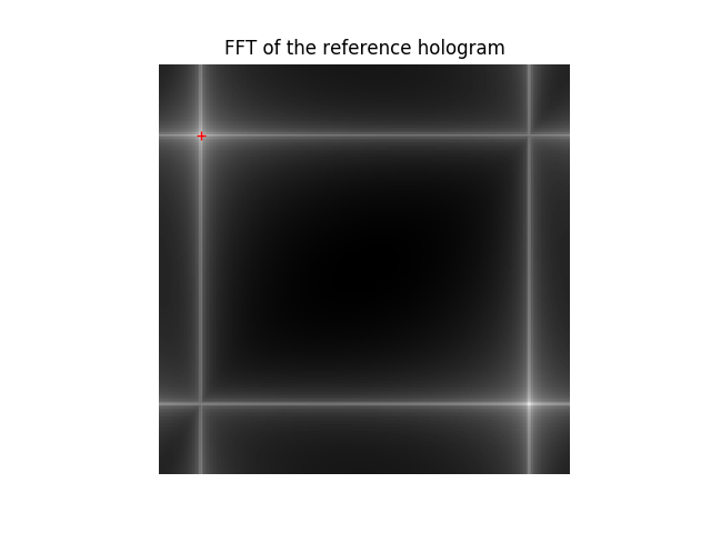
The reconstruction requires knowledge about the position of the sideband and the size of the sideband filter which will be used in the reconstruction. The position of the sideband can be estimated from the Fourier transform of the vacuum reference hologram:
# Plot FFT and the sideband position
plt.imshow(np.log(np.abs(np.fft.fft2(ref))))
plt.plot(26., 44., '+r')
plt.axis('off')
plt.title('FFT of the reference hologram')

# Define position
sb_position = [44, 26]
The radius of sideband filter is typically chosen as either half of the distance between the sideband and autocorrelation for strong phase objects or as one third of the distance for weak phase objects. Assuming a strong phase object, one can proceed as follows:
sb_size = np.hypot(sb_position[0], sb_position[1]) / 2.
Since in off-axis electron holography, the spatial resolution is determined by the interference fringe spacing rather than by the sampling of the original images, the reconstruction would typically involve changing the shape of the data. For medium magnification holography the size of the reconstructed images can be typically set to the size (diameter) of the sideband filter. (For high-resolution holography reconstruction, typically binning factors of 1-4 are used.) Therefore, the output shape can be defined as follows:
output_shape = (int(sb_size * 2), int(sb_size * 2))
Finally the HoloReconstructUDF class can be used to reconstruct the object and
reference holograms:
# Create reconstruction UDF:
holo_udf = HoloReconstructUDF(out_shape=output_shape,
                              sb_position=sb_position,
                              sb_size=sb_size)

# Reconstruct holograms, access data directly
w_holo = ctx.run_udf(dataset=dataset_holo,
                     udf=holo_udf)['wave'].data
w_ref = ctx.run_udf(dataset=dataset_ref,
                    udf=holo_udf)['wave'].data

# Correct object wave using reference wave
w = w_holo / w_ref

# Calculate plot phase shift and amplitude
amp_r = np.abs(w)
phase_r = np.angle(w)

# Plot amplitude
f, ax = plt.subplots(1, 2)
ax[0].imshow(amp)
ax[0].title.set_text('Input amplitude')
ax[0].set_axis_off()
ax[1].imshow(amp_r[0])
ax[1].title.set_text('Reconstructed amplitude')
ax[1].set_axis_off()
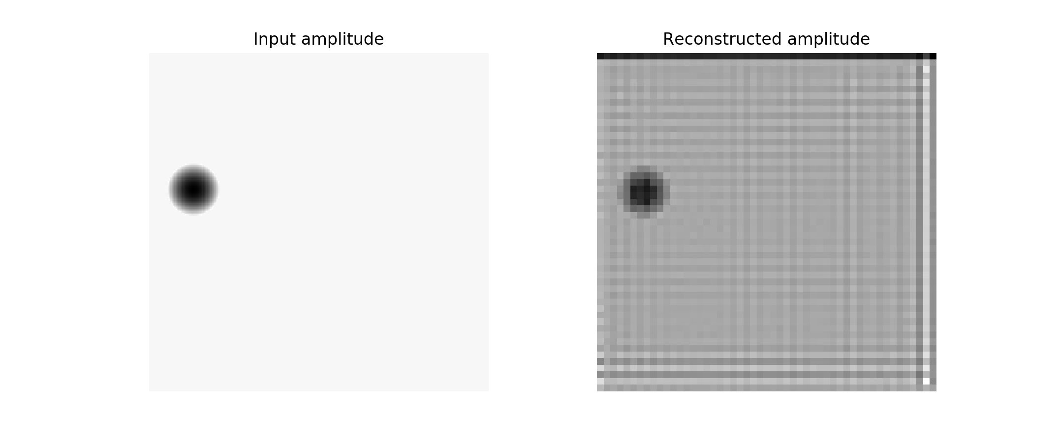
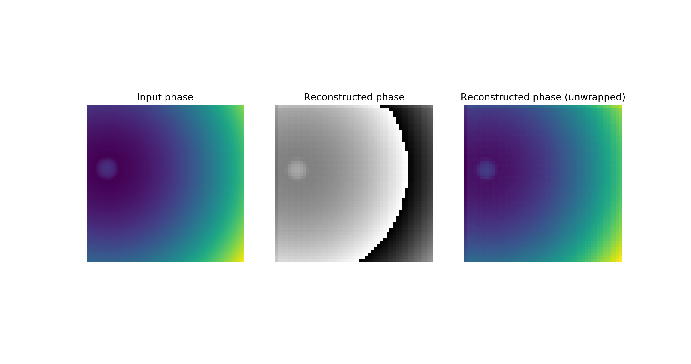
One sees that the reconstructed amplitude has artifacts due to digital Fourier processing. Those are typical for synthetic data. One of the ways to get synthetic data closer to the experimental would be adding noise. Comparing phase images, one should keep in mind that phase is typically wrapped in an interval \([0; 2\pi)\). To unwrap phase one can do the following:
from skimage.restoration import unwrap_phase

# Unwrap phase:
phase_unwrapped = unwrap_phase(phase_r[0])

# Plot
f, ax = plt.subplots(1, 3)
ax[0].imshow(phase, cmap='viridis')
ax[0].title.set_text('Input phase')
ax[0].set_axis_off()
ax[1].imshow(phase_r[0])
ax[1].title.set_text('Reconstructed phase')
ax[1].set_axis_off()
ax[2].imshow(phase_unwrapped, cmap='viridis')
ax[2].title.set_text('Reconstructed phase (unwrapped)')
ax[2].set_axis_off()
In addition to the capabilities demonstrated above, the HoloReconstructUDF
class can take smoothness of sideband (SB) filter as fraction of the SB size (sb_smoothness=0.05 is default).
Also, the precision argument can be used (precision=False) to reduce the calculation precision
to float32 and complex64 for the output. Note that depending of NumPy backend, even with reduced
precision the FFT function used in the reconstruction may internally calculate results with double
precision. In this case reducing precision will only affect the size of the output rather than the
speed of processing.