GUI usage

LiberTEM ships with a convenient web-based interface for quickly understanding a dataset through a selection of common analyses (virtual detectors, centre-of-mass, clustering etc).

Note

Note that the GUI is currently limited to 2D visualizations, which makes it adapted 4D-STEM imagery but not spectrum imaging such as STEM-EELS. If you have a need for display of 1D signals please file an issue.

Starting the GUI

You can the start the interface from the command line after activating the virtualenv or conda environment where LiberTEM is installed.

(libertem) $ libertem-server

In most situations this will automatically launch a webpage in your browser to start loading data and running analyses. If it didn’t open automatically, you can access it by default at http://localhost:9000.

Note

The GUI is tested to work on Firefox and Chromium-based browsers for now. If you cannot use a compatible browser for some reason, please file an issue.

It is also possible to connect to a libertem-server on a remote machine though this requires special configuration and depends on your network environment (see Configuring the LiberTEM server (Advanced)).

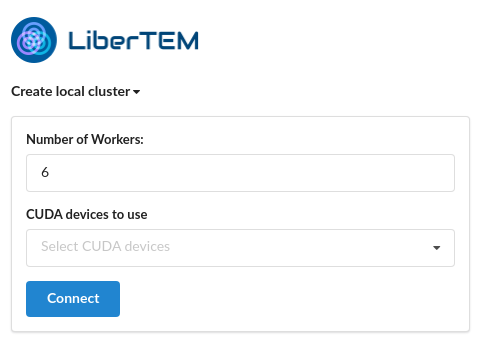
Create the local cluster

The first page in the GUI allows you to specify the compute resources the system will use to process your data (number of CPUs, GPUs etc). By default all available resources are selected, though you can reduce this if needed.

Note

Use of GPUs requires a working CuPy installation, see CuPy install for more information.

Opening data

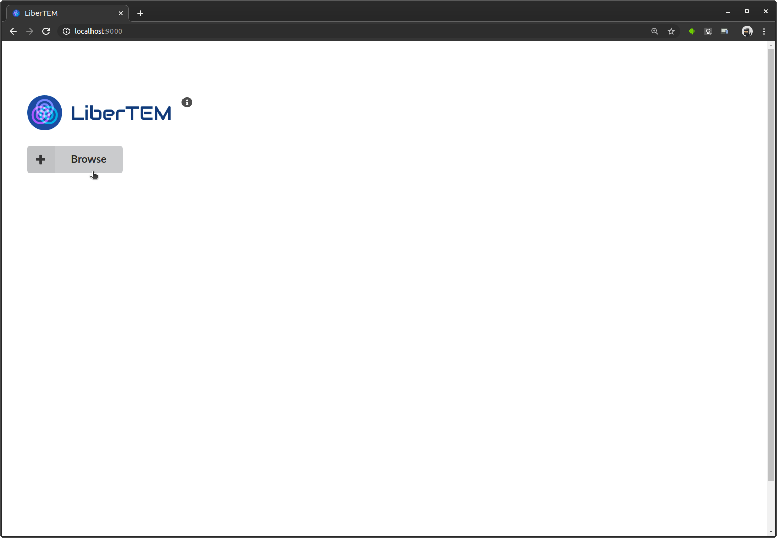
Next, LiberTEM shows a button to start browsing for available files. On a local machine that’s simply the local filesystem.

Note

See Sample Datasets for publicly available datasets.

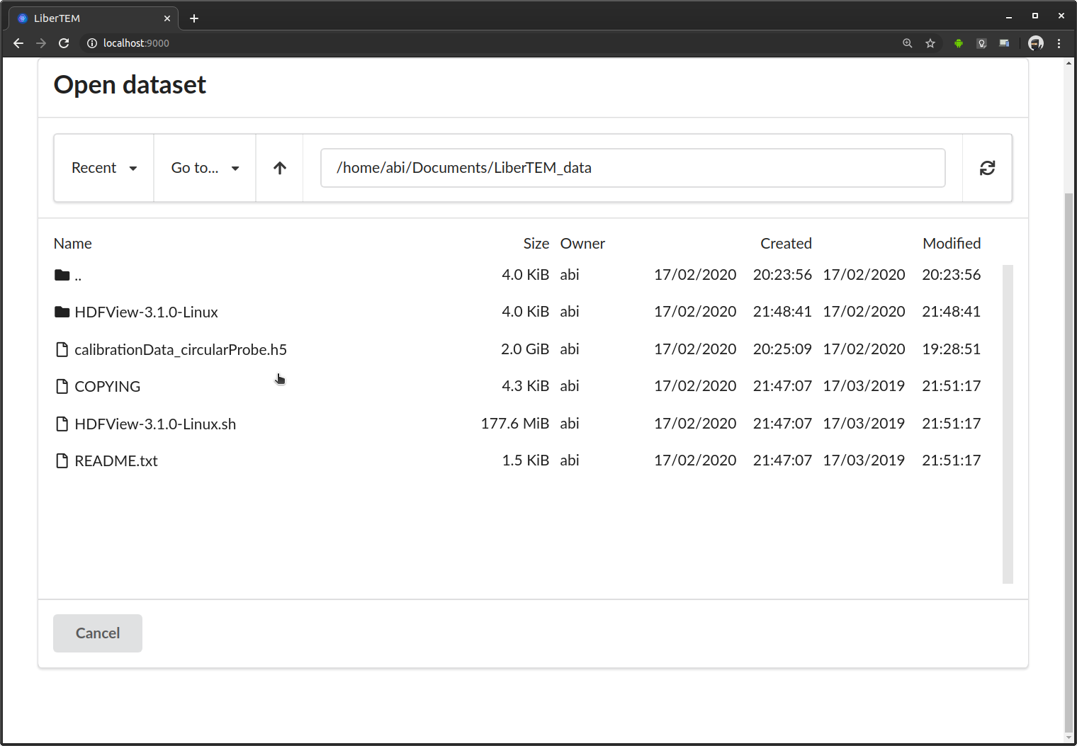
This opens the file browser dialogue. On top it shows the current directory, below it lists all files and subdirectories in that directory. You select an entry by clicking once on it. You can move up one directory with the “..” entry on top of the list. The file browser is still very basic. Possible improvements are discussed in Issue #83. Contributions are highly appreciated! This example opens an HDF5 file [ZMB+19].

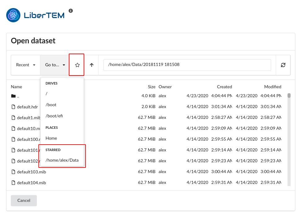
You can also bookmark locations you frequently need to access, using the star icon. The bookmarks are then found under “Go to…”.

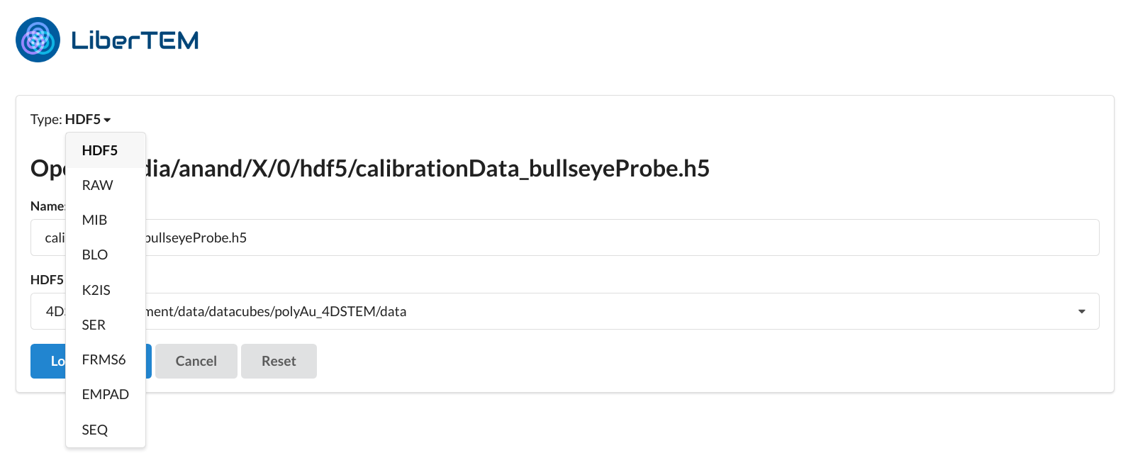
After selecting a file, you set the type in the drop-down menu at the top of the dialogue above the file name. After that you set the appropriate parameters that depend on the file type. Clicking on “Load Dataset” will open the file with the selected parameters. The interface and internal logic to find good presets based on file type and available metadata, validate the inputs and display helpful error messages is still work in progress. Contributions are highly appreciated!

See Loading using the GUI for more detailed instructions and format-specific information.

Running analyses

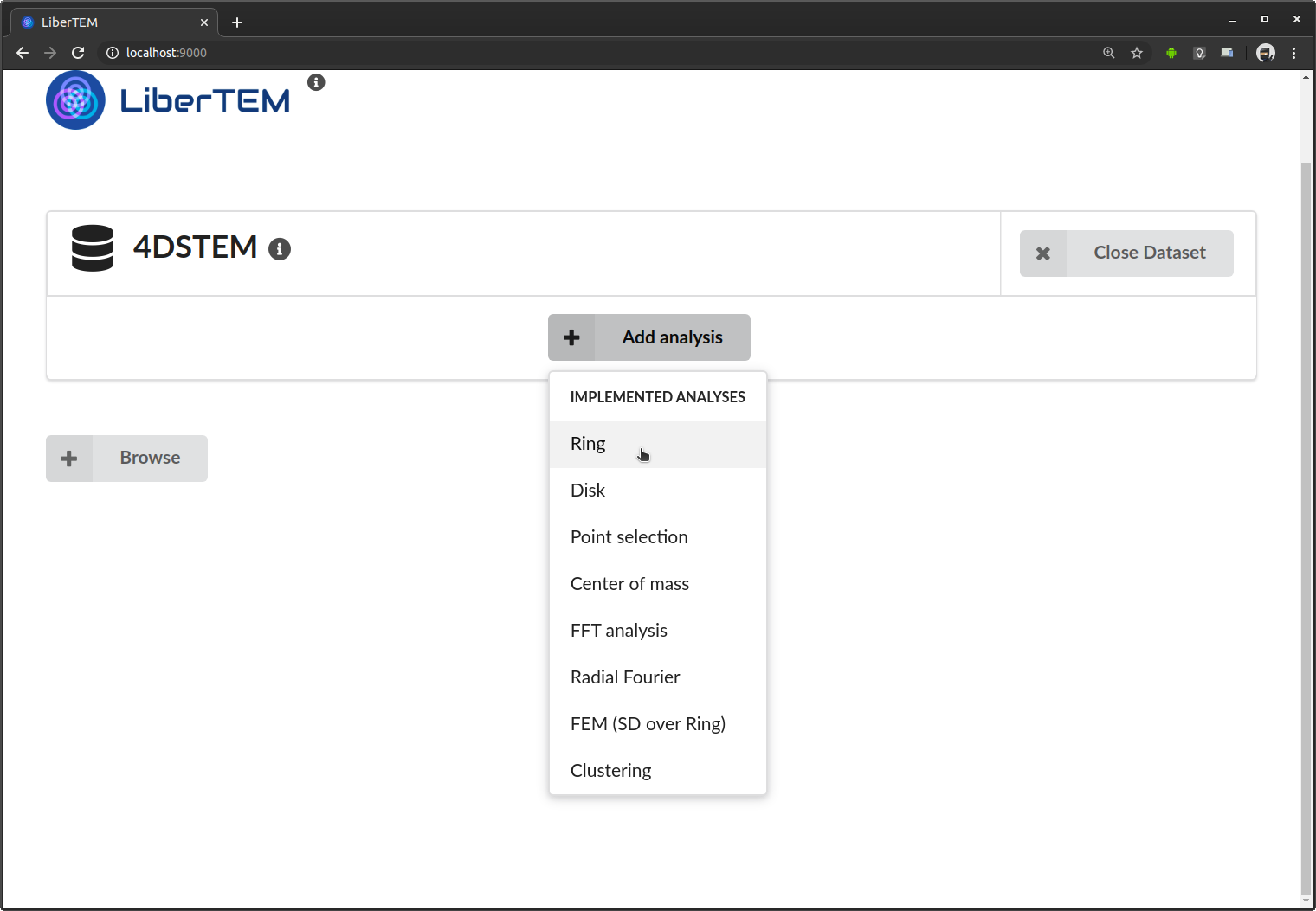
Once a dataset is loaded, you can add analyses to it. As an example we choose a “Ring” analysis, which implements a ring-shaped virtual detector.

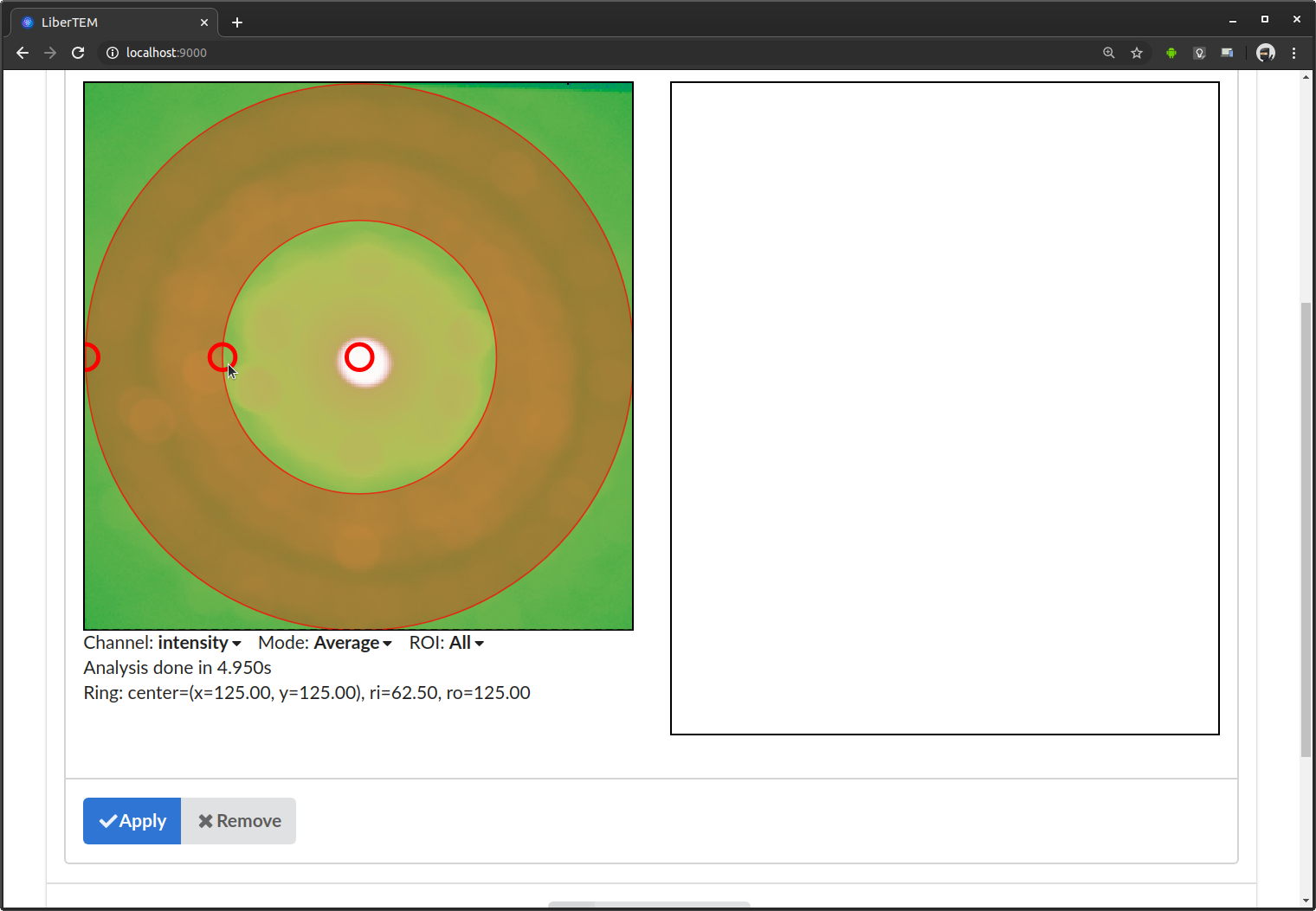
This analysis shows two views on your data: the two detector dimensions on the left, the scanning dimensions on the right, assuming a 4D-STEM dataset. For the general case, we also call the detector dimensions the signal dimensions, and the scanning dimensions the navigation dimensions. See also Concepts for more information on axes and coordinate system.

Directly after adding the analysis, LiberTEM starts calculating an average of all the detector frames. The average is overlaid with the mask representing the virtual detector. The view on the right will later show the result of applying the mask to the data. In the beginning it is empty. The first processing might take a while depending on file size and I/O performance. Fast SSDs and enough RAM to keep the working files in the file system cache are highly recommended for a good user experience.

You can adjust the virtual detector by dragging the handles in the GUI. Below it shows the parameters in numerical form. This is useful to extract positions, for example for scripting.

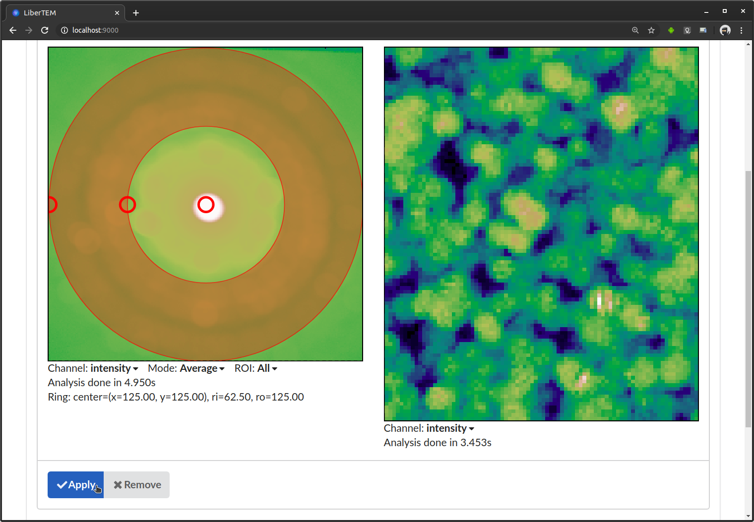
After clicking “Apply”, LiberTEM performs the calculation and shows the result in scan coordinates on the right side.

Instead of average, you can select “Standard Deviation”. This calculates standard deviation of all detector frames.

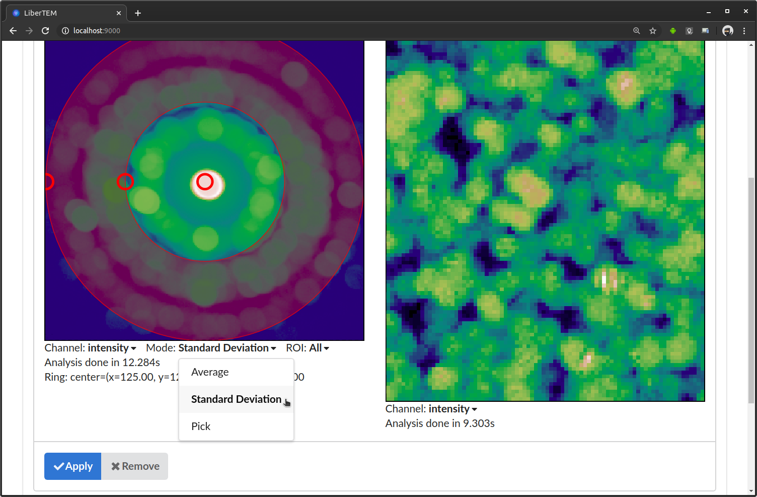
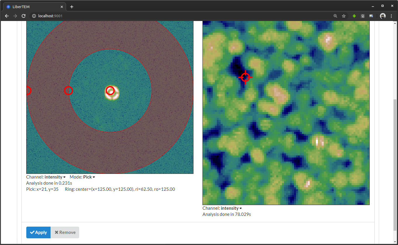
If you are interested in individual frames rather than the average, you can switch to “Pick” mode in the “Mode” drop-down menu directly below the detector window.

In “Pick” mode, a selector appears in the result frame on the right. You can drag it around with the mouse to see the frames live in the left window. The picked coordinates are displayed along with the virtual detector parameters below the frame window on the left.

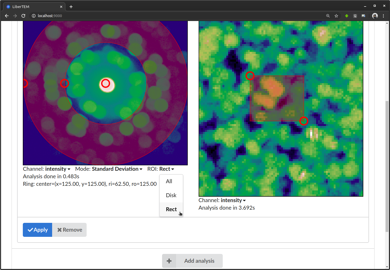
If you are interested in a limited region, the ROI dropdown provides the option to select a rectangular region. For example if you select “Rect”, the average/standard deviation is calculated over all images that lie inside selected rectangle. You can adjust the rectangle by dragging the handles in the GUI.

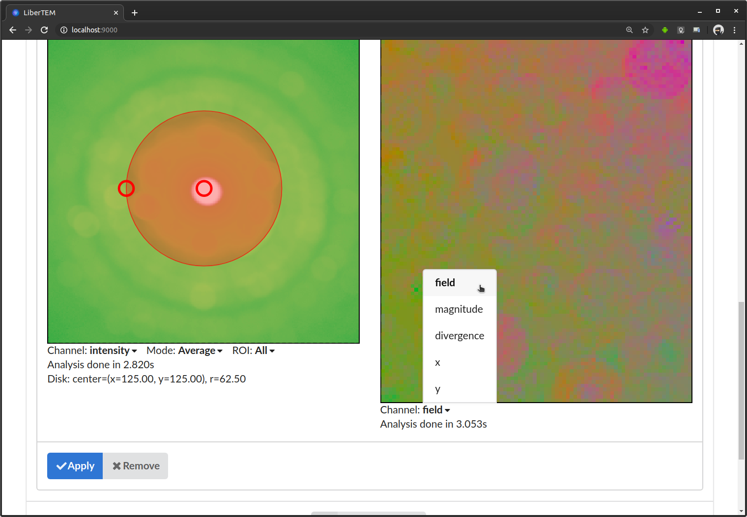
Some analyses, such as the Center of Mass (COM) analysis, can render the result in different ways. You can select different result channels in the “Channel” drop-down menu below the right window.

Downloading results

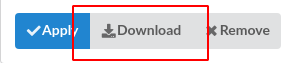
After an analysis has finished running, you can download the results. Clicking the download button below the analysis will open a dialog:

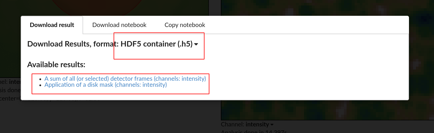
In the download dialog, you can choose between different file formats, and separately download the available results.

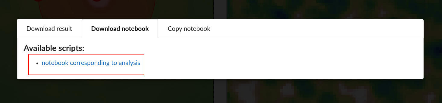
You can also download a Jupyter notebook corresponding to the analysis and continue working with the same parameters using scripting.

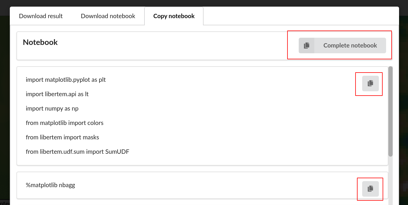
It’s also possible to copy individual cells of Jupyter notebook directly from GUI, with an option to copy the complete source code.

Keyboard controls

You can use arrow keys to change the coordinate parameters of any analysis. To do this, click on the handle you want to modify, and then use the arrow keys to move the handle. Hold shift to move in larger steps.

Application-specific documentation

For more applications, like strain mapping and crystallinity analysis, please see the Applications section.

Configuring the LiberTEM server (Advanced)

The LiberTEM GUI is based on a client-server architecture. To use the LiberTEM GUI, you need to have the server running on the machine where your data is available. For using LiberTEM from Python scripts, this is not necessary, see Python API.

By default, this starts the server on http://localhost:9000, which you can verify by the log output:

[2018-08-08 13:57:58,266] INFO [libertem.web.server.main:886] listening on localhost:9000

To modify the configuration of the server (address, port, autorization etc.), the libertem-server has a number of options available:

Usage: libertem-server [OPTIONS]

Options:
  -h, --host TEXT                 host on which the server should listen on
                                  [default: localhost]
  -p, --port INTEGER              port on which the server should listen on,
                                  [default: 9000]
  -d, --local-directory TEXT      local directory to manage dask-worker-space
                                  files
  -b, --browser / -n, --no-browser
                                  enable/disable opening the browser
  -c, --cpus INTEGER              number of cpu worker processes to
                                  use,[default: select in GUI]
  -g, --gpus INTEGER              number of gpu worker processes to
                                  use,[default: select in GUI]
  -o, --open-ds TEXT              dataset to preload via URL action
  -l, --log-level TEXT            set logging level. Default is 'info'.
                                  Allowed values are 'critical', 'error',
                                  'warning', 'info', 'debug'.
  -t, --token-path PATH           path to a file containing a token for
                                  authenticating API requests
  --preload TEXT                  Module, file or code to preload on workers,
                                  for example HDF5 plugins. Can be specified
                                  multiple times. See also
                                  https://docs.dask.org/en/stable/customize-
                                  initialization.html#preload-scripts for the
                                  behavior with Dask workers (current
                                  default)and https://libertem.github.io/Liber
                                  TEM/reference/dataset.html#hdf5 for
                                  information on loading HDF5 files that
                                  depend on custom filters.
  --insecure                      Allow connections from non-localhost without
                                  token authorization. Applies only when
                                  combined with --host <address> (use
                                  `--insecure -h 0.0.0.0` to accept any
                                  connection)
  --snooze-timeout FLOAT          Free resources after periods of no activity,
                                  in minutes. Depending on your system, re-
                                  starting these resources might take some
                                  time, so typical values are 10 to 30
                                  minutes.
  --help                          Show this message and exit.

New in version 0.4.0: --browser / --no-browser option was added, open browser by default.

New in version 0.6.0: -l, --log-level was added.

New in version 0.8.0: -t, --token-path was added and -h, --host was re-enabled.

New in version 0.9.0: --preload and --insecure were added.

New in version 0.13.0: --cpus <int> and --gpus <int> were added to preconfigure the cluster resources

New in version 0.13.0: --open-ds <path> was added to preconfigure the dataset opened when connecting to the server

New in version 0.14.0: --snooze-timeout was added, keeping the old behaviour by default.

To access LiberTEM remotely, you can use use SSH forwarding or our Jupyter integration, if you already have JupyterHub or JupyterLab set up on a server.