Phase-change materials
Phase-change materials are some of the most promising materials for data-storage applications. In this application section, a pixelated STEM dataset from a AgInSbTe phase-change material specimen will be processed. Distinguishing between amorphous and crystalline regions can be hard in microstructure analysis with 4-D-STEM because of low contrast between them during the two most common method of visualization: bright and dark field imaging. The main difference of pixelated diffraction patterns for each of the beam positions the presence of additional (non zero-order) diffraction peaks in crystalline frames, while the amorphous frames have only the zero-order peak. Detection of the positions of additional peaks for all frames of crystalline regions will allow gaining information on the crystal structure.
Next, methods to distinguish crystalline and amorphous regions in phase-change materials will be described.
Note
See Phase-change materials reference for the API reference.
Crystallinity map
First, two different types of the regions, crystalline (low resistance) and amorphous (high resistance), should be distinguished. Crystalline regions are characterized by the presence of additional non-zero diffraction peaks on diffraction image, while the diffraction image (the frame) of amorphous regions contains only the zero-order diffraction peak on a diffuse scattering background. The presence of additional periodic diffraction peaks leads to differences in the Fourier spectrum of the crystalline frames compared to amorphous frames in the intermediate frequency range. Integration of all frames Fourier spectra over a ring (in intermediate frequency range) and using the result of the integration as intensity for each position for sample visualization (similar to virtual dark field image, but in Fourier space) allows distinguishing amorphous and crystalline regions of the sample.
GUI use:
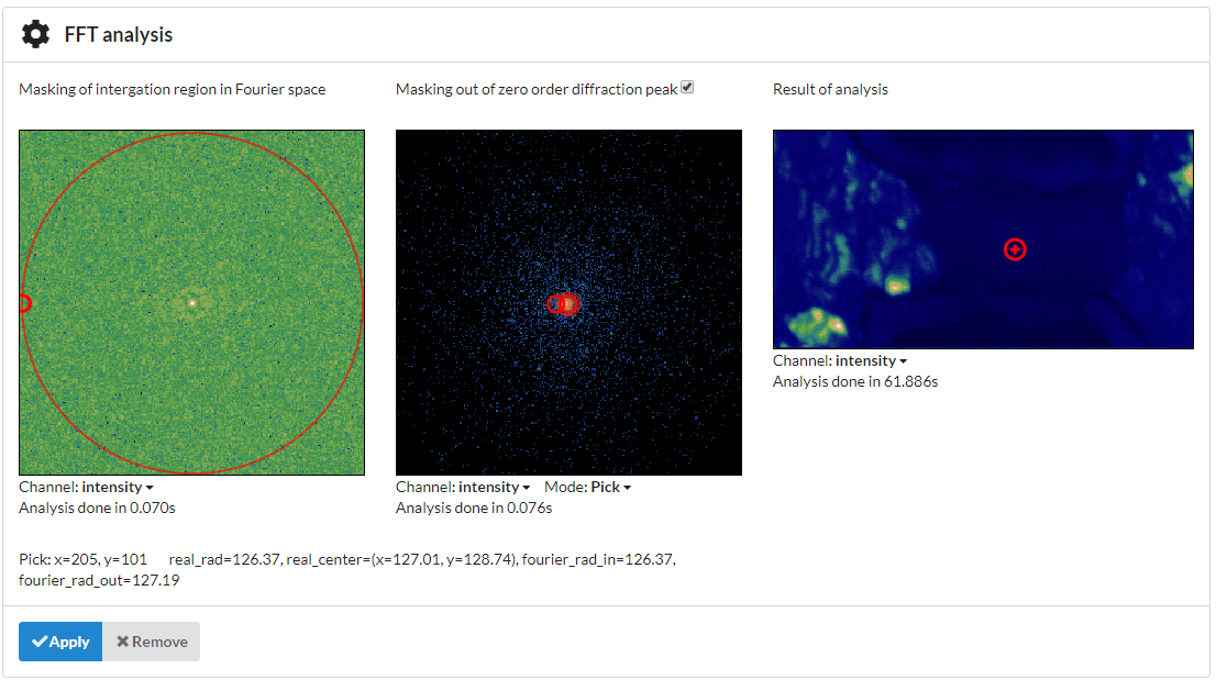
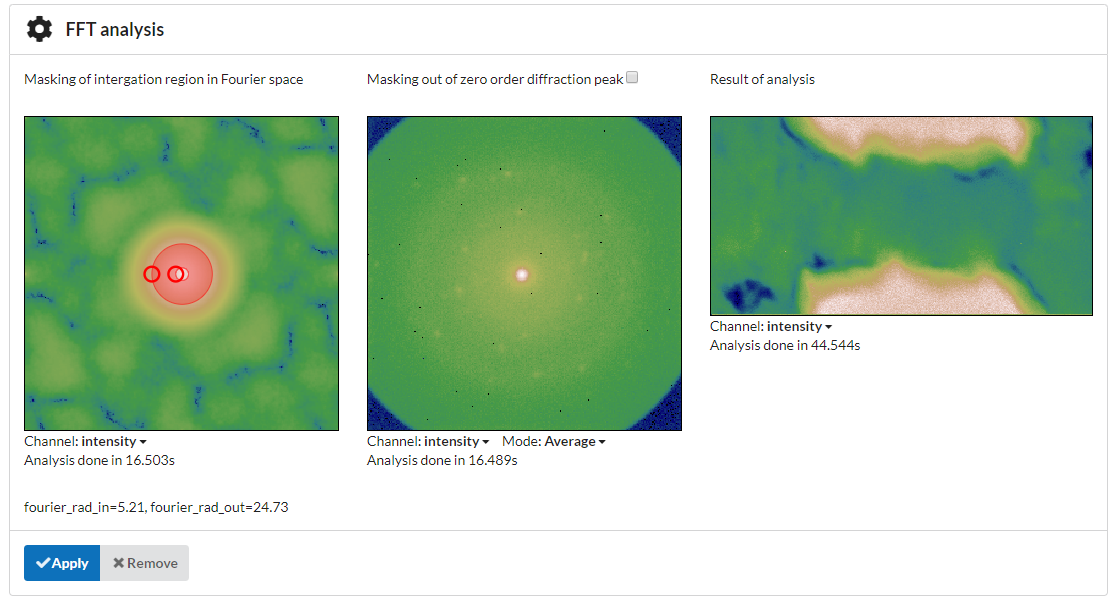
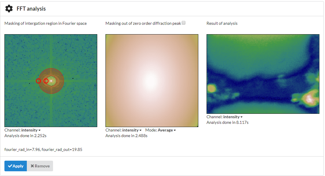
You can select “FFT Fourier” from the “Add Analysis” menu in the GUI to obtain crystallinity map with high contrast between crystalline and amorphous regions.
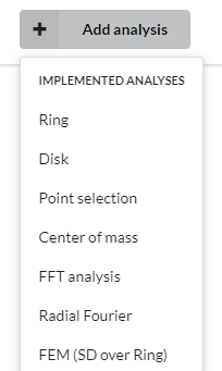
Use the checkbox in the middle if you would like to enable/disable of masking of zero-order peak out. In case of enabling zero-order diffraction peak removal: use the controls on the middle to position the disk-shaped selector over the region of average frame you’d like to mask out. Then, adjust the radii on the left to position the ring-shaped selector over the region of the average of frames spectra you’d like to integrate over and then click “Apply”.
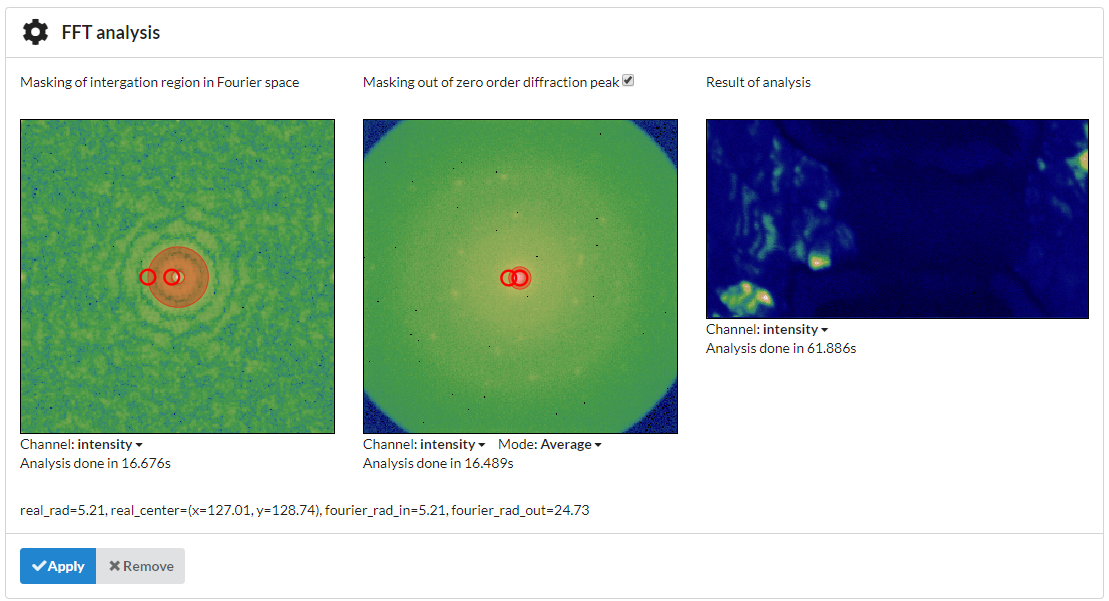
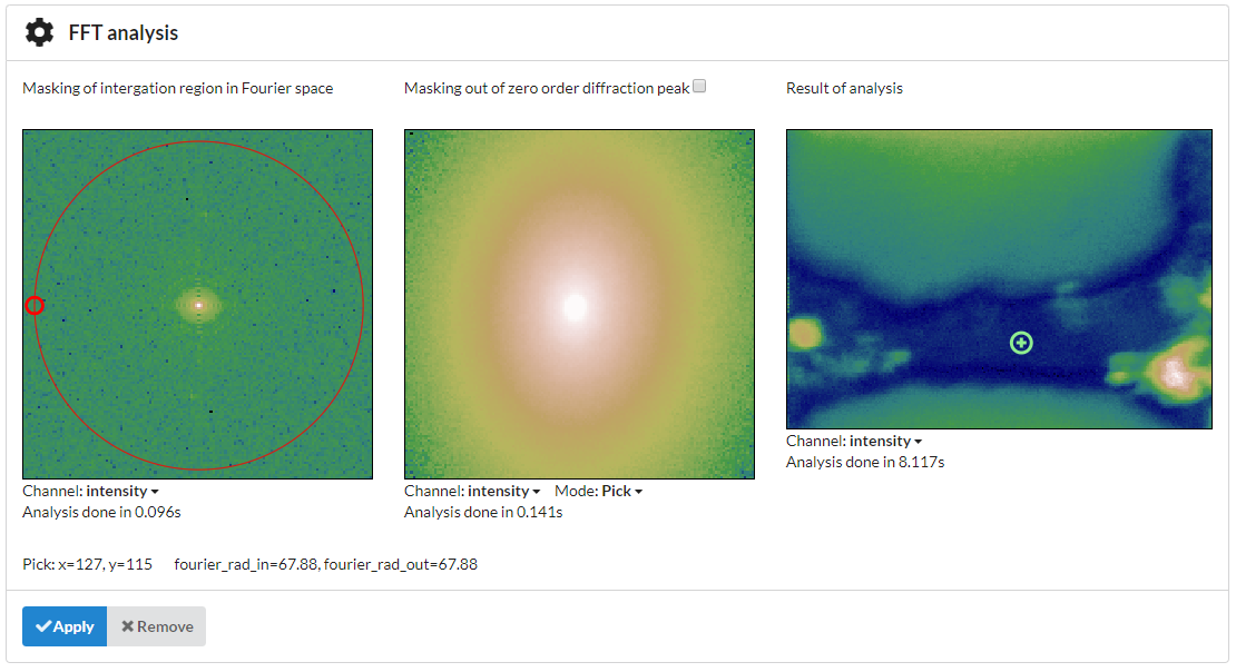
In the right side, the resulting image will be generated. To check the quality of the detection you can use pick mode which is located under the middle image. In the case of correct parameters settings, crystalline regions will be brighter than amorphous.
Crystalline frame:
Amorphous frame:
Tips for enabling/disabling of zero-order diffraction peak removal:
In case of the sharp and bright zero-order peak you will need to mask it out, as it described above (spectrum of such a peak will be a 2d sinc function which will spread all over the frames spectra)
So, the crystallinity map will not provide any contrast.
But, in the case of sinc shaped zero-order peak, you do not need to remove it. The influence of it will be presented in low-frequency range and will be masked out during the integration region choosing
Crystalline frame:

Amorphous frame:
Clustering
New in version 0.3.0.
To further categorize the crystalline regions according to their lattice orientation, clustering, based on non-zero diffraction peaks positions, can be used. The scripting interface allows to cluster membrane, amorphous and crystalline regions with different lattice orientation in a more efficient way, taking into account regions of interests. To look at full analysis follow this link to a Jupyter notebook.
GUI use:
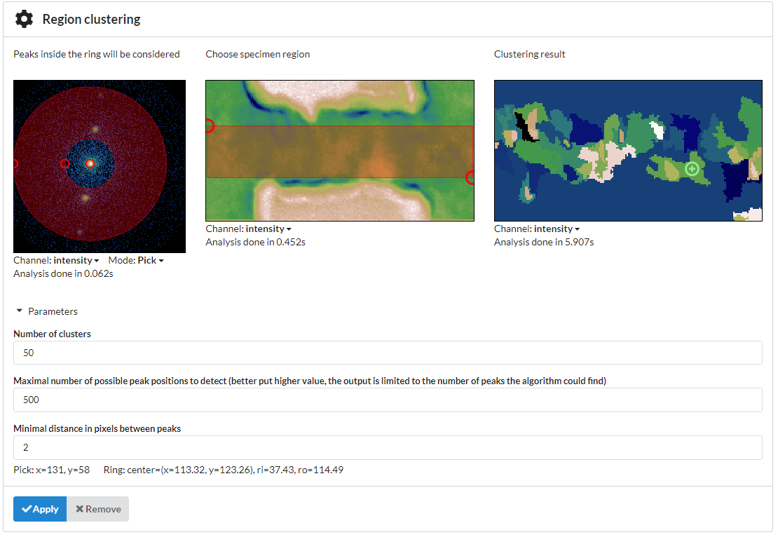
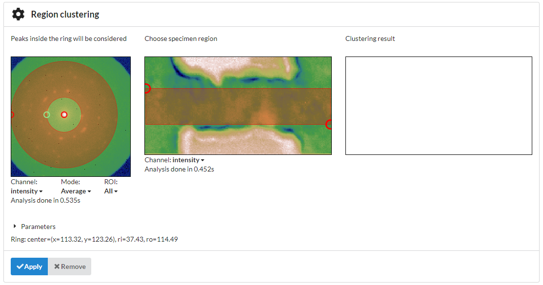
To make preliminary analysis for parameters choice and a brief look at the result, you can select “Clustering” from the “Add Analysis” menu in the GUI.
Then you can choose the region in the navigation space in the middle to select the standard deviation (SD) calculation region (recommendation: try to select as much of the specimen you can, avoiding zones without usable data, such as membrane or vacuum). The frame regions which will have higher intensity in the standard deviation image will be assumed as possible positions of non-zero order diffraction peaks. Adjust the position of the ring and its radii in the left side to select the region for detecting peaks and click “Apply”. Then, for each of coordinates of the peaks on SD image, the decision about the presence or absence of a peak at this position for each frame will be made. Next, as a result, the feature vector will be generated for each frame to further use in clustering.
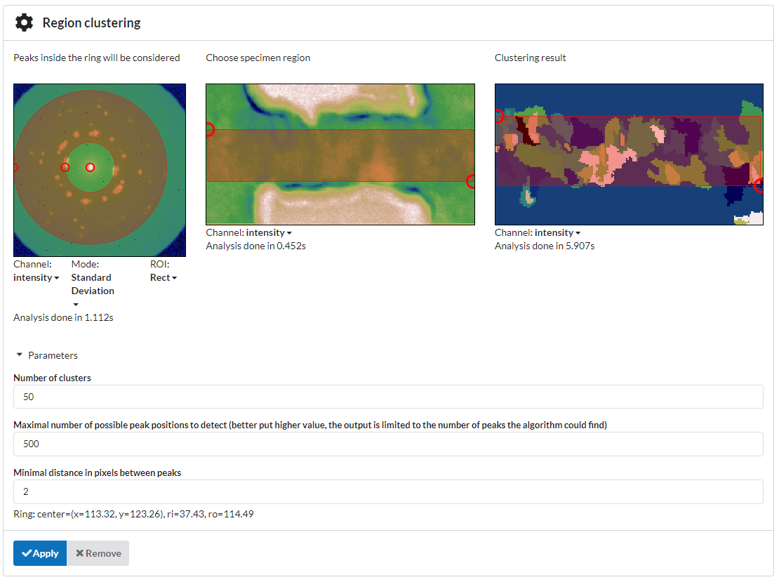
After the first result will be shown, you can readjust the region of peak detection (in the left side), SD calculation region (in the middle) and parameters, which are hidden in the parameters section. For radii readjustment, you can use SD over ROI mode. To see the correct ROI, use the “SD over ROI (rect) mode”. To choose ROI for feature vector calculation and clustering, use the middle section.
You can check the clustering result by using Pick mode.
Example of cluster with one lattice orientation:
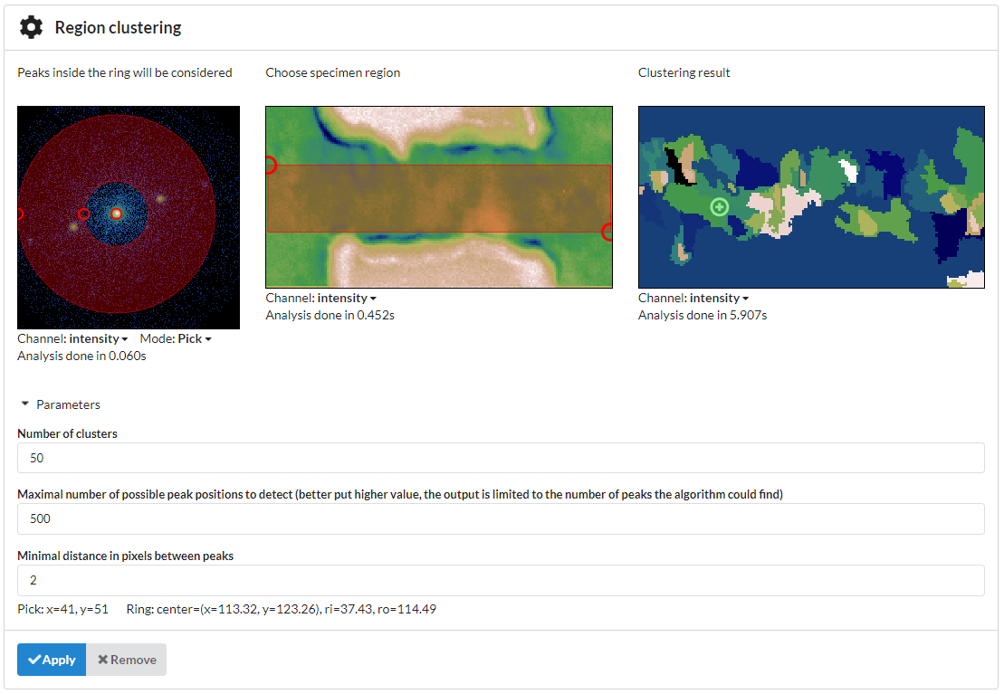
Example of cluster with another lattice orientation: