Amorphous materials

Note

See Fluctuation EM and Radial Fourier Analysis for API references

LiberTEM offers methods to determine the local order or crystallinity of amorphous and nanocrystalline materials.

Fluctuation EM

The diffraction pattern of amorphous materials show a characteristic ring of intensity around the zero-order diffraction peak that is a result of near-range ordering of the atoms in the material. Any local ordering within the interaction volume of beam and sample will lead to increased “speckle”, i.e. intensity fluctuations within this ring, since regions with local ordering will diffract the beam to preferred directions similar to a crystal. For Fluctuation EM [GT97], the standard deviation within this ring is calculated to obtain a measure of this local ordering.

GUI use

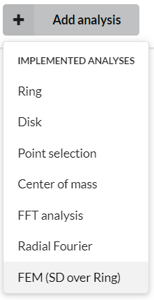
You can select FEM from the “Add Analysis” menu in the GUI to add a Fluctuation EM Analysis.

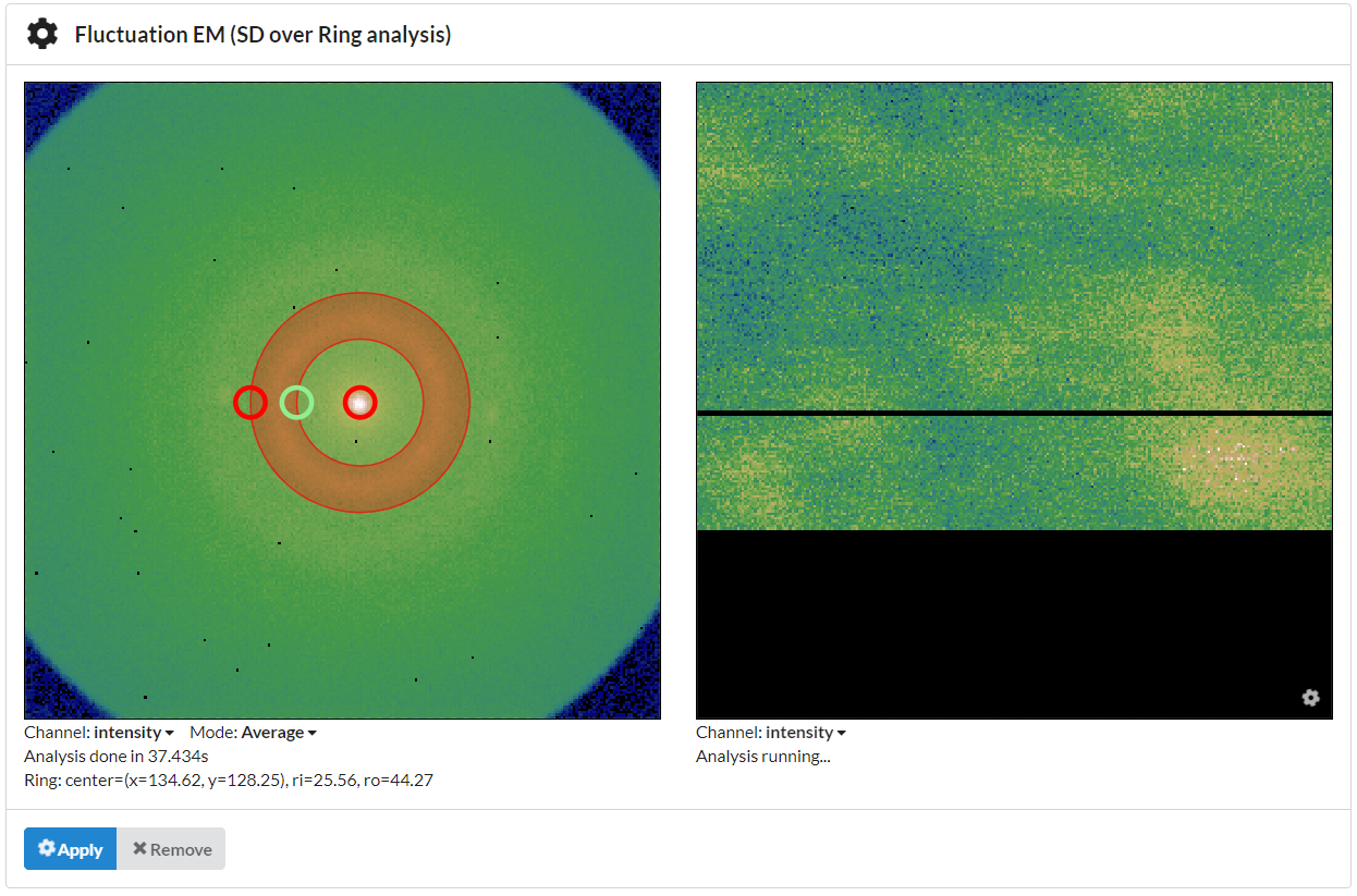
Use the controls on the left to position the ring-shaped selector over the region you’d like to analyze and then click “Apply”.

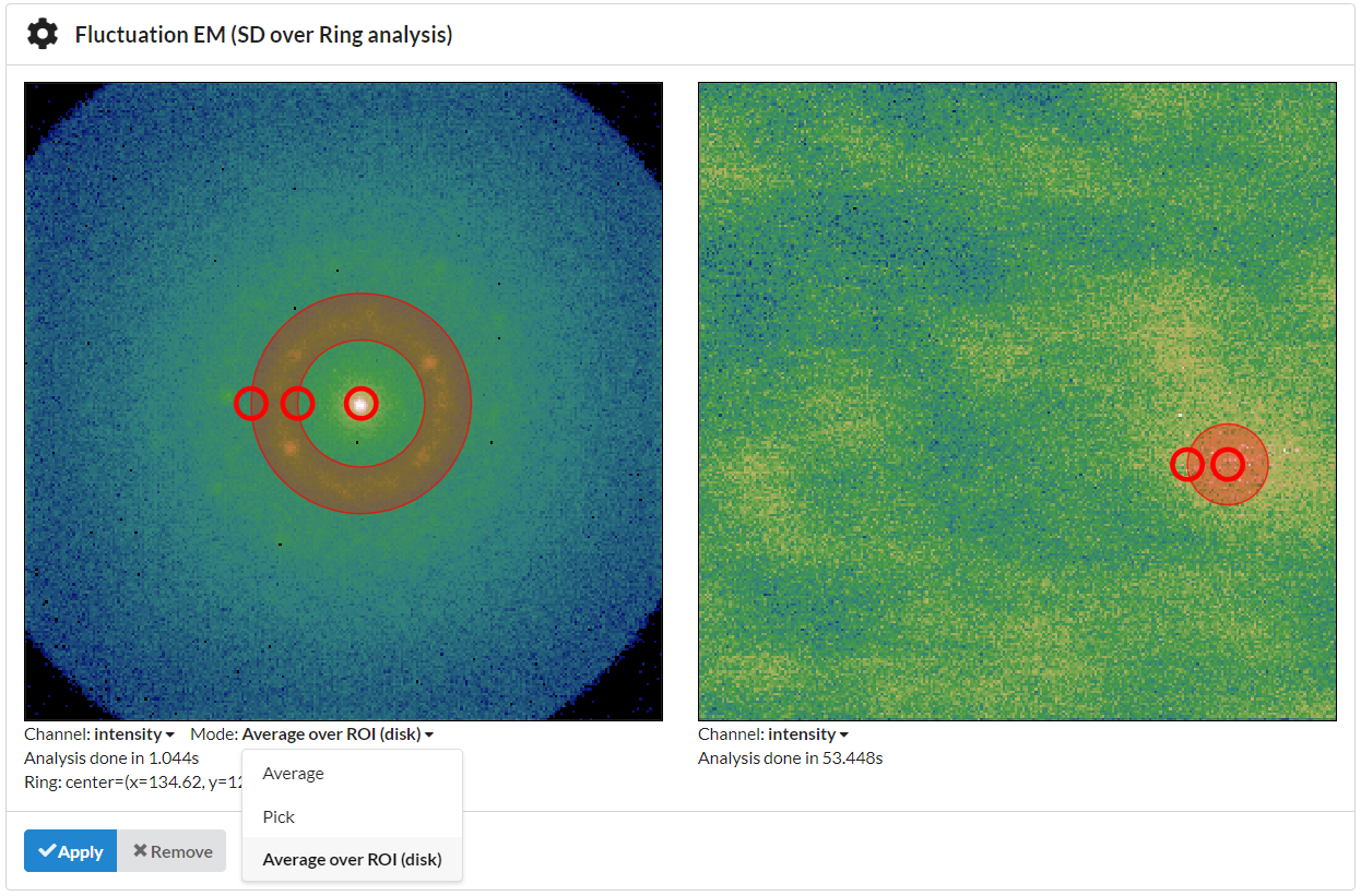
Pick mode or average over ROI comes in handy to inspect individual frames or regions of interest:

Sample data: Metallic glass courtesy of Shuai Wei <shuai.wei@physik.rwth-aachen.de>, RWTH Aachen; Alexander Kuball, Universität des Saarlandes; Hongchu Du <h.du@fz-juelich.de>, ER-C, Forschungszentrum Jülich.

Scripting interface

LiberTEM supports this with the FEMUDF and run_fem() method.

Radial Fourier Series

• Radial Fourier Analysis scripting example
  • Calculate a spectrum for the entire scan as a function of radius
  • Summing the absolutes of all non-zero components
  • We can do a radial profile of any order.
  • The zero order component is just the radial sum.
  • We analyze which coefficients are present in that ring
  • We calculate maps for selected orders across the scan
  • The phase gives information about orientation
  • We determine which order is predominant

Fluctuation EM doesn’t evaluate the spatial distribution of intensity. It only works if enough intensity accumulates in each pixel so that local ordering leads to larger intensity variations than just random noise, i.e. if statistical variations from shot noise average out and variations introduced by the sample dominate.

If most of the detector pixels are only hit with one electron or none, the standard deviation between detector positions in a region of interest is the same, even if pixels that received electrons are spatially close, while other regions received no intensity. That means Fluctuation EM doesn’t produce contrast between amorphous and crystalline regions if the detector has a high resolution, and/or if only low intensity is scattered into the region of interest.

The Radial Fourier Series Analysis solves this problem by calculating a Fourier series in a ring-shaped region instead of just evaluating the standard deviation. The reference [LinWongJiang+14] describes a previous application of this method as a descriptor for feature extraction from images. The angle of a pixel relative to the user-defined center point of the diffraction pattern is used as a phase angle for the Fourier series.

Since diffraction patterns usually show characteristic symmetries, the strength of the Fourier coefficients of orders 2, 4 and 6 highlight regions with crystalline order for even the lowest intensities. With the relationship between variance in real space and power spectral density in frequency space, the sum of all coefficients that are larger than zero is equivalent to the standard deviation, i.e. Fluctuation EM. Only summing coefficients from lower orders corresponds Fluctuation EM on a smoothened dataset.

The phase angle of selected coefficients, for example first or second order, can be used for in-plane orientation mapping similar to [POT+19].

Please note that this method is new and experimental and still needs to be validated further. If you are interested in helping us with applications and validations, that would be highly appreciated!

GUI use

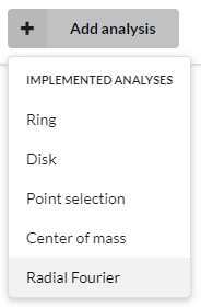
You can select “Radial Fourier” from the “Add Analysis” menu in the GUI to add a Radial Fourier Series Analysis.

Use the controls on the left to position the ring-shaped selector over the region you’d like to analyze and then click “Apply”.

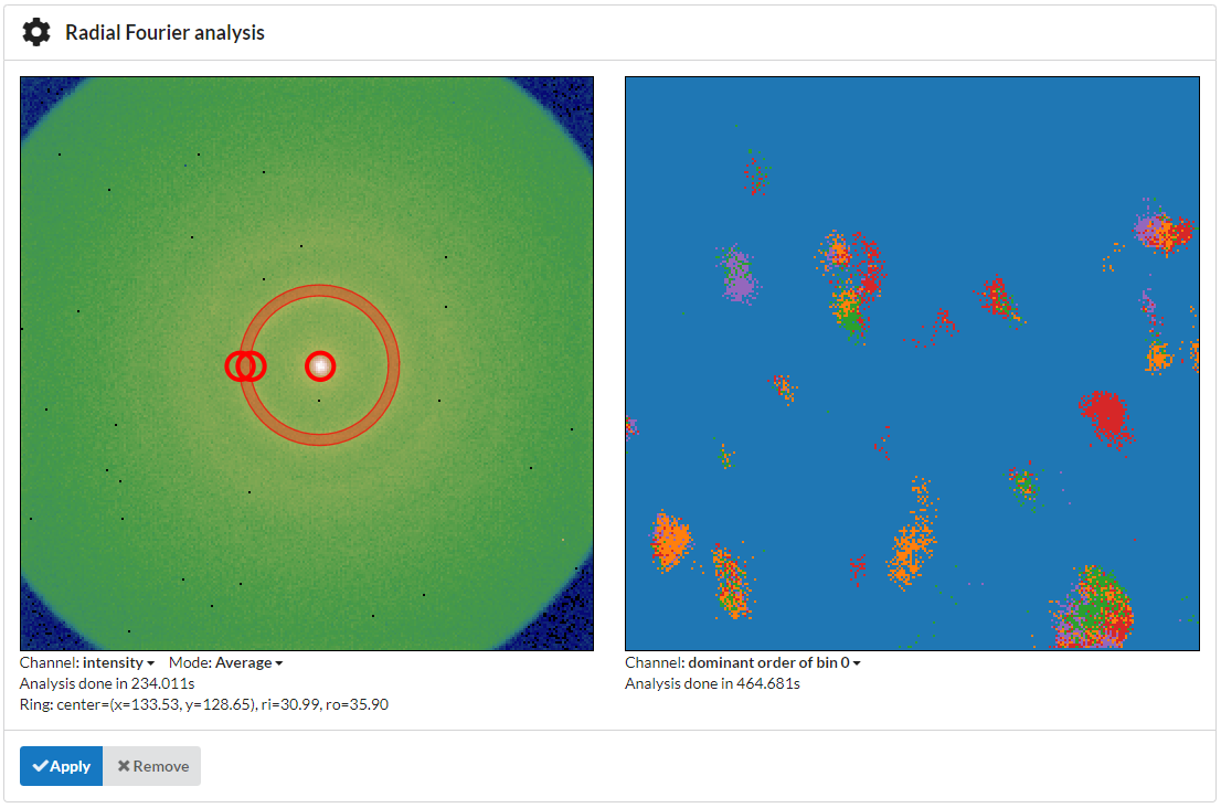
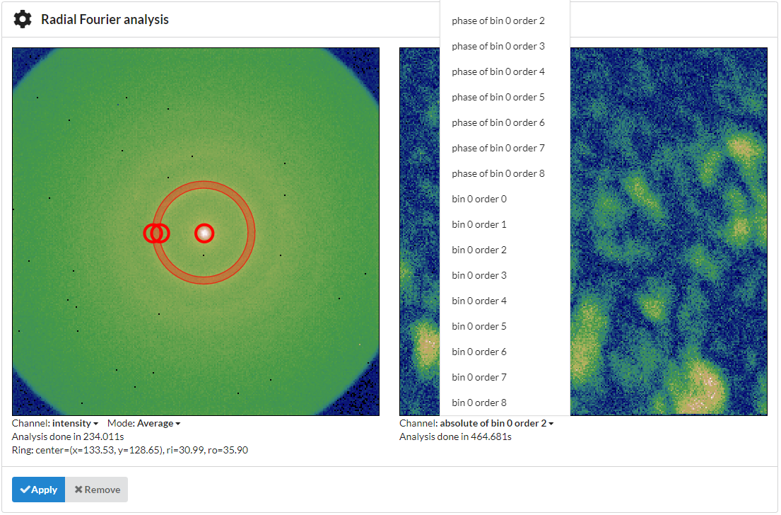
Under the right-hand side image you can select the channel to display. Available are predominant order, absolute value, phase angle and a cubehelix vector field visualization of the complex number. The orders larger than zero are all plotted on the same range and are normalized by the zero-order component for each scan position to make the components comparable and eliminate the influence of absolute intensity variations in the visual display.

You can select entries with the arrow keys on the keyboard in case the menu is outside the browser window. Your help with a more user-friendly GUI implementation would be highly appreciated!

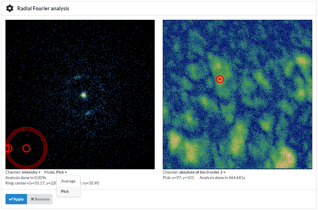
Pick mode comes in handy to inspect individual frames:

Sample data: Metallic glass courtesy of Shuai Wei <shuai.wei@physik.rwth-aachen.de>, RWTH Aachen; Alexander Kuball, Universität des Saarlandes; Hongchu Du <h.du@fz-juelich.de>, ER-C, Forschungszentrum Jülich.

Scripting interface

The scripting interface create_radial_fourier_analysis() and RadialFourierAnalysis allows to calculate more than one bin at a time and influence the number of orders that are calculated. It relies on the sparse matrix back-end for ApplyMasksUDF and allows to calculate many orders for many bins at once with acceptable efficiency.

Having a fine-grained analysis with many orders calculated as a function of radius allows for a number of additional processing and analysis steps. Follow this link to a Jupyter notebook.

Reference

See Fluctuation EM and Radial Fourier Analysis for API references!