Live plotting for LiberTEM UDFs
This example demonstrates the live plotting feature of LiberTEM that is introduced in release 0.7.0. It can update a plot with new results while LiberTEM processing is running.
The data can be downloaded at https://doi.org/10.5281/zenodo.5113449.
This notebook requires additional packages bqplot, bqplot_image_gl and ipywidgets. See also https://ipywidgets.readthedocs.io/en/stable/user_install.html#installing-in-classic-jupyter-notebook in case the plots don’t show.
[1]:
%matplotlib widget
[2]:
import os
import matplotlib.pyplot as plt
import matplotlib.colors
import ipywidgets
import IPython
import numpy as np

import libertem.api as lt
from libertem.udf import UDF
from libertem.udf.raw import PickUDF
from libertem.viz.mpl import MPLLive2DPlot
from libertem.viz.bqp import BQLive2DPlot
Plot classes
Currently, LiberTEM implements three back-ends for live plotting:
libertem.viz.mpl.MPLLive2DPlotwith amatplotlibback-end. It is the default sincematplotlibis the most popular and mature plotting package for Python. It requires about 100-200 ms to display or update a plot, which only allows a few updates per second.libertem.viz.bqp.BQLive2DPlotwith abqplot_image_glback-end. It is much faster thanmatplotliband can easily keep up with the full update rate of LiberTEM for a smoother and more responsive display.libertem.viz.gms.GMSLive2DPlotfor plotting within Digital Micrograph, Gatan Microscopy Suite. This only works using the Python scripting of recent GMS releases and is not demonstrated here.
Additional plotting back-ends can be implemented by deriving from libertem.viz.base.Live2DPlot.
Here we change the default class for live plotting to BQLive2DPlot and then change it back right away by assigning to the plot_class property of the LiberTEM Context object.
[3]:
# We set the Context to use BQLive2DPlot for live plotting
ctx = lt.Context(plot_class=BQLive2DPlot)

# We change it right back to the default MPLLive2DPlot
ctx.plot_class = MPLLive2DPlot
[4]:
data_base_path = os.environ.get("TESTDATA_BASE_PATH", "/home/alex/Data/")
ds = ctx.load("auto", path=os.path.join(data_base_path, "20200518 165148/default.hdr"))

# This internal method is used here to artificially create more partitions than necessary
# for better demonstration of live plotting on machines with few cores.
# This reduces performance, should NOT be used in production and can change without
# notice in future releases.
ds.set_num_cores(32)
Demo UDFs
We implement three simple user-defined functions (UDFs) to demonstrate the various features and options for live plotting. They calculate a map of the navigation space with sum and maximum, a map of the signal space with sum and maximum, and a global maximum.
See https://libertem.github.io/LiberTEM/udf.html for more information on UDFs.
[5]:
class DemoNavUDF(UDF):
    def get_result_buffers(self):
        return {
            'nav_sum': self.buffer(kind='nav', dtype='float32'),
            'nav_max': self.buffer(kind='nav', dtype='float32'),
        }

    def process_frame(self, frame):
        self.results.nav_sum[:] = np.sum(frame)
        self.results.nav_max[:] = np.max(frame)


class DemoSigUDF(UDF):
    def get_result_buffers(self):
        return {
            'sig_sum': self.buffer(kind='sig', dtype='float32'),
            'sig_max': self.buffer(kind='sig', dtype='float32'),
        }

    def process_frame(self, frame):
        self.results.sig_sum += frame
        np.maximum(self.results.sig_max, frame, out=self.results.sig_max)

    def merge(self, dest, src):
        dest.sig_sum += src.sig_sum
        np.maximum(dest.sig_max, src.sig_max, out=dest.sig_max)


class DemoSingleUDF(UDF):
    def get_result_buffers(self):
        return {
            'maximum': self.buffer(kind='single', dtype='float32'),
        }

    def process_frame(self, frame):
        self.results.maximum[:] = np.maximum(self.results.maximum, np.max(frame))

    def merge(self, dest, src):
        dest.maximum[:] = np.maximum(dest.maximum, src.maximum)
The UDFs are instantiated and stored in a list for subsequent use.
[6]:
udfs = [DemoNavUDF(), DemoSigUDF(), DemoSingleUDF()]
Plot all plottable channels
Note how Context.run_udf() can execute several UDFs in one pass since release 0.7.0 by passing a list or tuple of UDFs.
By setting plots=True you can plot all channels that have a 2D shape after applying np.squeeze. The DemoSingleUDF is not plotted since its only channel maximum is a single value. This triggers a warning.
[7]:
# NBVAL_IGNORE_OUTPUT
# (output is ignored in nbval run because it somehow doesn't work with widgets)
res = ctx.run_udf(dataset=ds, udf=udfs, plots=True)
Select specific channels
We can specify which channels should be plotted by passing a nested list with channel names for each of the UDFs as the plots parameter.
[8]:
# NBVAL_IGNORE_OUTPUT
# (output is ignored in nbval run because it somehow doesn't work with widgets)
res = ctx.run_udf(dataset=ds, udf=udfs, plots=[['nav_sum'], ['sig_sum', 'sig_max']])
Apply a function to a channel
Together with the channel name we can specify a function to apply to the channel before plotting. This can plot a channel that doesn’t work with default plotting by transforming it into something plottable. Here we demonstrate this with the single-valued maximum channel.
The same channel can be plotted several times with a different function. This is particularly useful to plot the absolute value and the phase angle for complex numbers: ('chan', np.abs), ('chan', np.angle). Here we demonstrate this with thresholding.
[9]:
# Just some thresholding for demonstration
def larger(x):
    return x > 9.3e4

def smaller(x):
    return x < 9e4
[10]:
# NBVAL_IGNORE_OUTPUT
# (output is ignored in nbval run because it somehow doesn't work with widgets)
plot_list=[
    ['nav_sum', ('nav_sum', larger), ('nav_sum', smaller)],
    [],
    [('maximum', lambda x: x.reshape((1, 1)))]
]

res = ctx.run_udf(dataset=ds, udf=udfs, plots=plot_list)
Custom plot setup
If we want to have more control over the plots and their layout, we can instantiate plots separately and pass them to run_udf() via the plots parameter. This also allows to set additional parameters such as the title. Note how MPLLive2DPlot passes additional keyword arguments, in this case the color map cmap and the norm, to matplotlib.pyplot.imshow.
The UDF passed to the live plot via the udf parameter has to be the same instance that is later run in run_udf() to ensure that results are assigned to the correct plot.
[11]:
live_plot = MPLLive2DPlot(
    dataset=ds,
    udf=udfs[1],
    # We add 1 for log scale display since there are zeros in the result
    channel=('sig_sum', lambda x: 1 + x),
    title="1 + x, log scaled display",
    # These parameters are passed to imshow()
    cmap='inferno',
    norm=matplotlib.colors.LogNorm()
)
[12]:
# NBVAL_IGNORE_OUTPUT
# (output is ignored in nbval run because it somehow doesn't work with widgets)
live_plot.display()
# We can access and modify the matplotlib objects, in this case to add a color bar
live_plot.fig.colorbar(live_plot.im_obj)
[12]:
<matplotlib.colorbar.Colorbar at 0x7ff08c39de10>
[13]:
# Run the UDF, showing live results in the plot above
res = ctx.run_udf(dataset=ds, udf=udfs, plots=[live_plot])
Gridded display
Here we use bqplot and arrange the plots in a grid. The same method can also be used with MPLLive2DPlot if the output method of matplotlib is switched to use ipywidgets. Just install ipympl, replace %matplotlib nbagg at the top of the notebook with %matplotlib widget and restart the kernel.
Note that at the time of writing this notebook, a MPLLive2DPlot combined with display method “widget” will only update live if it is created and displayed separately, not if this is done automatically in run_udf() .
[14]:
# NBVAL_IGNORE_OUTPUT
# (output is ignored in nbval run because it somehow doesn't play nice with bqplot)

live_plots = [
    BQLive2DPlot(dataset=ds, udf=udfs[0], channel='nav_sum'),
    BQLive2DPlot(dataset=ds, udf=udfs[0], channel=('nav_sum', larger)),
    BQLive2DPlot(dataset=ds, udf=udfs[0], channel=('nav_sum', smaller)),
    BQLive2DPlot(dataset=ds, udf=udfs[1], channel='sig_sum'),
    BQLive2DPlot(dataset=ds, udf=udfs[1], channel='sig_max'),
    BQLive2DPlot(dataset=ds, udf=udfs[2], channel=('maximum', lambda x: x.reshape((1, 1)))),
]

outputs = []

for p in live_plots:
    # We capture the display of the widget with ipywidgets.Output() to arrange it later
    output = ipywidgets.Output()
    with output:
        p.display()
        # Some bqplot-specific tweaks to reduce white space between plots
        p.figure.fig_margin={'top': 50, 'bottom': 0, 'left': 25, 'right': 25}
        p.figure.layout.height = '300px'
    outputs.append(output)
[15]:
# NBVAL_IGNORE_OUTPUT
# Display the captured outputs in a grid
ipywidgets.VBox([
    ipywidgets.HBox(outputs[:3]),
    ipywidgets.HBox(outputs[3:]),
])
[15]:
What it looks like
The gridded layout is currently not preserved when saving the notebook. This PNG shows a screenshot:
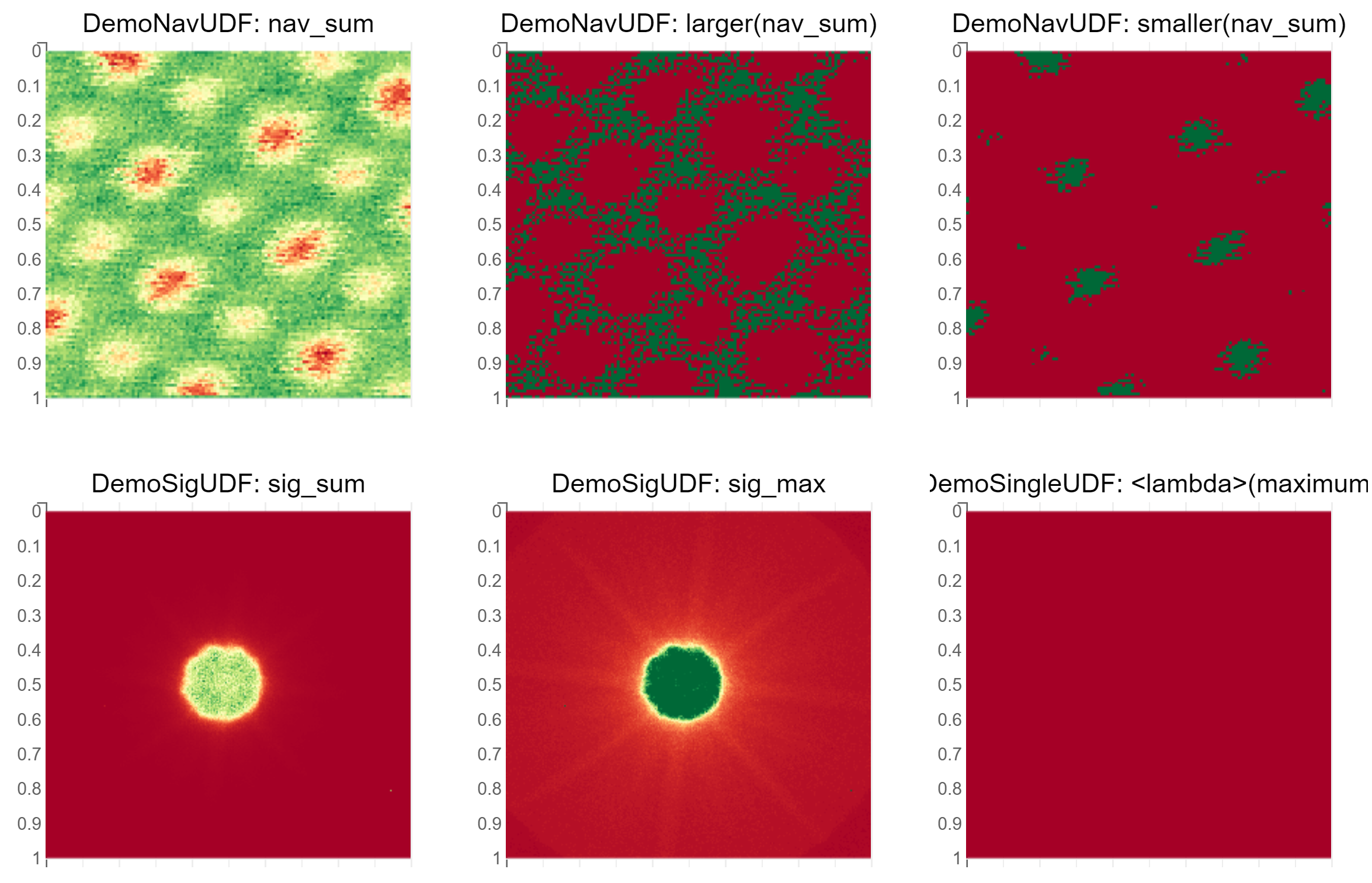
[16]:
res = ctx.run_udf(dataset=ds, udf=udfs, plots=live_plots)
User-defined plotting
In some cases one may want to plot results that are based on combining several channels of a UDF. As a specific example, when strain mapping with https://libertem.github.io/LiberTEM-blobfinder/ one may want to plot the angle between the a and b vectors in the fit result. Live2DPlot allows to pass a callable as the channel argument that will receive a complete UDF result together with a damage buffer that indicates which part of the navigation space has already been processed.
The callable is expected to return an ndarray together with damage that indicates the positions in the result that hold valid data. If the result is derived from kind='nav' buffers, the damage parameter of the function can be passed through. If the result is derived from other buffers, i.e. the entire result array contains valid data, the function can just return True for the damage.
Here we will plot the ratio between sum and max for demonstration purposes.
[17]:
def nav_ratio(udf_result, damage):
    # We use the damage to exclude invalid data
    # Avoid divide by 0
    where = damage & (np.abs(udf_result['nav_max'].data) > 1e-12)
    result = np.divide(
        udf_result['nav_sum'].data,
        udf_result['nav_max'].data,
        where=where
    )
    return result, damage

def sig_ratio(udf_result, damage):
    # Avoid divide by 0
    where = np.abs(udf_result['sig_max'].data) > 1e-12
    result = np.divide(
        udf_result['sig_sum'].data,
        udf_result['sig_max'].data,
        where=where
    )
    return result, True
[18]:
# NBVAL_IGNORE_OUTPUT
# (output is ignored in nbval run because it somehow doesn't work with widgets)
live_plots = [
    MPLLive2DPlot(dataset=ds, udf=udfs[0], channel=nav_ratio),
    MPLLive2DPlot(dataset=ds, udf=udfs[1], channel=sig_ratio),
]

for p in live_plots:
    p.display()
    p.fig.colorbar(p.im_obj)
[19]:
res = ctx.run_udf(dataset=ds, udf=udfs, plots=live_plots)
Region of interest (ROI)
The shape of result buffers can depend on the ROI in some cases. The most notable example is libertem.udf.raw.PickUDF. For that reason we should pass the ROI to the constructor of Live2DPlot subclasses if the UDFs will be run with a ROI.
[20]:
roi = ds.roi[0, 0]
pick_udf = PickUDF()
[21]:
# NBVAL_IGNORE_OUTPUT
# (output is ignored in nbval run because it somehow doesn't work with widgets)
# This just works, the ROI is handled correctly internally
ctx.run_udf(dataset=ds, udf=pick_udf, roi=roi, plots=True)
[21]:
{'intensity': <BufferWrapper kind=single dtype=uint8 extra_shape=(1, 256, 256)>}
[22]:
# NBVAL_IGNORE_OUTPUT
# (output is ignored in nbval run because it somehow doesn't work with widgets)
# Here we have to pass the ROI
# If this was omitted, the PickUDF would allocate memory for the entire dataset and the plot would try to display that!
live_plot_pick = MPLLive2DPlot(dataset=ds, udf=pick_udf, roi=roi, channel='intensity')
live_plot_pick.display()
[23]:
ctx.run_udf(dataset=ds, udf=pick_udf, roi=roi, plots=[live_plot_pick])
[23]:
{'intensity': <BufferWrapper kind=single dtype=uint8 extra_shape=(1, 256, 256)>}
Note that the first axis of the result of PickUDF matches the number of entries in the ROI that are True. If this is a single one, this axis is “squeezed out” with default plotting. If functions are used to transform the result, this is the responsibility of the user. If more than one entry in the ROI is True, the result can’t be plotted with default methods since it can’t be squeezed to 2D anymore.
[24]:
# NBVAL_RAISES_EXCEPTION
# Error, wrong shape!
ctx.run_udf(dataset=ds, udf=pick_udf, roi=roi, plots=[[('intensity', lambda x: x)]])
---------------------------------------------------------------------------
TypeError                                 Traceback (most recent call last)
Cell In[24], line 3
      1 # NBVAL_RAISES_EXCEPTION
      2 # Error, wrong shape!
----> 3 ctx.run_udf(dataset=ds, udf=pick_udf, roi=roi, plots=[[('intensity', lambda x: x)]])

File /cachedata/alex/source/LiberTEM/.tox/notebooks_gen/lib/python3.11/site-packages/libertem/api.py:1030, in Context.run_udf(self, dataset, udf, roi, corrections, progress, backends, plots, sync)
   1028 with tracer.start_as_current_span("Context.run_udf"):
   1029     if sync:
-> 1030         return self._run_sync(
   1031             dataset=dataset,
   1032             udf=udf,
   1033             roi=roi,
   1034             corrections=corrections,
   1035             progress=progress,
   1036             backends=backends,
   1037             plots=plots,
   1038             iterate=False,
   1039         )
   1040     else:
   1041         return self._run_async(
   1042             dataset=dataset,
   1043             udf=udf,
   (...)   1049             iterate=False,
   1050         )

File /cachedata/alex/source/LiberTEM/.tox/notebooks_gen/lib/python3.11/site-packages/libertem/api.py:1273, in Context._run_sync(self, dataset, udf, roi, corrections, progress, backends, plots, iterate)
   1271 if enable_plotting:
   1272     with tracer.start_as_current_span("prepare_plots"):
-> 1273         plots = self._prepare_plots(udfs, dataset, roi, plots)
   1275 if corrections is None:
   1276     corrections = dataset.get_correction_data()

File /cachedata/alex/source/LiberTEM/.tox/notebooks_gen/lib/python3.11/site-packages/libertem/api.py:1518, in Context._prepare_plots(self, udfs, dataset, roi, plots)
   1506     for channel in udf_channels:
   1507         p0 = self.plot_class(
   1508             dataset,
   1509             udf=udf,
   (...)   1516             ),
   1517         )
-> 1518         p0.display()
   1519         plots.append(p0)
   1520 return plots

File /cachedata/alex/source/LiberTEM/.tox/notebooks_gen/lib/python3.11/site-packages/libertem/viz/mpl.py:93, in MPLLive2DPlot.display(self)
     91 with ui_events() as poll:
     92     self.fig, self.axes = plt.subplots()
---> 93     self.im_obj = self.axes.imshow(self.data, **self.kwargs)
     94     # Set values compatible with log norm
     95     self.im_obj.norm.vmin = 1

File /cachedata/alex/source/LiberTEM/.tox/notebooks_gen/lib/python3.11/site-packages/matplotlib/__init__.py:1524, in _preprocess_data.<locals>.inner(ax, data, *args, **kwargs)
   1521 @functools.wraps(func)
   1522 def inner(ax, *args, data=None, **kwargs):
   1523     if data is None:
-> 1524         return func(
   1525             ax,
   1526             *map(cbook.sanitize_sequence, args),
   1527             **{k: cbook.sanitize_sequence(v) for k, v in kwargs.items()})
   1529     bound = new_sig.bind(ax, *args, **kwargs)
   1530     auto_label = (bound.arguments.get(label_namer)
   1531                   or bound.kwargs.get(label_namer))

File /cachedata/alex/source/LiberTEM/.tox/notebooks_gen/lib/python3.11/site-packages/matplotlib/axes/_axes.py:5982, in Axes.imshow(self, X, cmap, norm, aspect, interpolation, alpha, vmin, vmax, colorizer, origin, extent, interpolation_stage, filternorm, filterrad, resample, url, **kwargs)
   5979 if aspect is not None:
   5980     self.set_aspect(aspect)
-> 5982 im.set_data(X)
   5983 im.set_alpha(alpha)
   5984 if im.get_clip_path() is None:
   5985     # image does not already have clipping set, clip to Axes patch

File /cachedata/alex/source/LiberTEM/.tox/notebooks_gen/lib/python3.11/site-packages/matplotlib/image.py:685, in _ImageBase.set_data(self, A)
    683 if isinstance(A, PIL.Image.Image):
    684     A = pil_to_array(A)  # Needed e.g. to apply png palette.
--> 685 self._A = self._normalize_image_array(A)
    686 self._imcache = None
    687 self.stale = True

File /cachedata/alex/source/LiberTEM/.tox/notebooks_gen/lib/python3.11/site-packages/matplotlib/image.py:653, in _ImageBase._normalize_image_array(A)
    651     A = A.squeeze(-1)  # If just (M, N, 1), assume scalar and apply colormap.
    652 if not (A.ndim == 2 or A.ndim == 3 and A.shape[-1] in [3, 4]):
--> 653     raise TypeError(f"Invalid shape {A.shape} for image data")
    654 if A.ndim == 3:
    655     # If the input data has values outside the valid range (after
    656     # normalisation), we issue a warning and then clip X to the bounds
    657     # - otherwise casting wraps extreme values, hiding outliers and
    658     # making reliable interpretation impossible.
    659     high = 255 if np.issubdtype(A.dtype, np.integer) else 1

TypeError: Invalid shape (1, 256, 256) for image data
[25]:
# NBVAL_IGNORE_OUTPUT
# (output is ignored in nbval run because it somehow doesn't work with widgets)
# Works, we squeeze the extra axis out
ctx.run_udf(dataset=ds, udf=pick_udf, roi=roi, plots=[[('intensity', lambda x: x.squeeze())]])
[25]:
{'intensity': <BufferWrapper kind=single dtype=uint8 extra_shape=(1, 256, 256)>}
[26]:
# We have a ROI with two entries
roi_two = ds.roi[(0, -1), (0, -1)]
[27]:
# No plot shown since the result is 3D now
ctx.run_udf(dataset=ds, udf=pick_udf, roi=roi_two, plots=True)
[27]:
{'intensity': <BufferWrapper kind=single dtype=uint8 extra_shape=(2, 256, 256)>}
[ ]: