LiberTEM UDFs

%matplotlib inline

import os
import matplotlib.pyplot as plt
import libertem.api as lt
import numpy as np

ctx = lt.Context()

Specifying the dataset

Most formats can be loaded using the "auto" type, but some may need additional parameters.

See the loading data section of the LiberTEM docs for details.

data_base_path = os.environ.get("TESTDATA_BASE_PATH", "/home/alex/Data/")

ds = ctx.load("auto", path=os.path.join(data_base_path, "01_ms1_3p3gK.hdr"))

After loading, some information is available in the diagnostics attribute:

ds.diagnostics

[{'name': 'Bits per pixel', 'value': '12'},
 {'name': 'Data kind', 'value': 'u'},
 {'name': 'Layout', 'value': '(1, 1)'},
 {'name': 'Partition shape', 'value': '(2075, 256, 256)'},
 {'name': 'Number of partitions', 'value': '32'},
 {'name': 'Number of frames skipped at the beginning', 'value': 0},
 {'name': 'Number of frames ignored at the end', 'value': 0},
 {'name': 'Number of blank frames inserted at the beginning', 'value': 0},
 {'name': 'Number of blank frames inserted at the end', 'value': 0}]

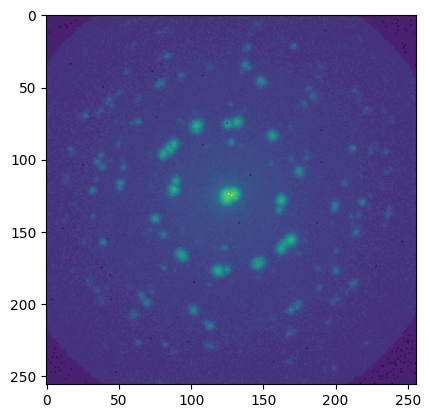
Standard analyses: virtual detector

A standard analysis to run on 4D STEM data is to apply a virtual detector. Here, we define a ring detector, with radii in pixels:

ring = ctx.create_ring_analysis(dataset=ds, ri=60, ro=70)

The analysis can be run with the Context.run method:

ring_res = ctx.run(ring, progress=True)
ring_res

[<AnalysisResult: intensity>, <AnalysisResult: intensity_log>]

As the analysis mirrors what the web GUI does, we have to access the data using the raw_data attribute, as we would get a viusalized result otherwise. Here we do the visualization ourselves using matplotlib:

plt.figure()
plt.imshow(ring_res.intensity.raw_data)

<matplotlib.image.AxesImage at 0x7f4a2ecc57b0>

Simple UDF definition

User-defined funtions provide a way for you to implement your own data processing functionality. As a very simple example, we define a function that just sums up the pixels of each frame:

def sum_of_pixels(frame):
    return np.sum(frame)

The easiest way to run this on the data is to use the Context.map function:

res_pixelsum_1 = ctx.map(dataset=ds, f=sum_of_pixels, progress=True)
res_pixelsum_1

<BufferWrapper kind=nav dtype=float32 extra_shape=()>

The result is of type BufferWrapper, but can be used by any function that expects a numpy array, for example for plotting it:

plt.figure()
plt.imshow(res_pixelsum_1)

<matplotlib.image.AxesImage at 0x7f4a1ff597b0>

The Context.map function is a shortcut for implementing very easy mapping over data, in a frame-by-frame fashion. The longer way of writing this would be as follows:

from libertem.udf import UDF


class SumOfPixels(UDF):
    def get_result_buffers(self):
        return {
            'sum_of_pixels': self.buffer(kind='nav', dtype='float32')
        }

    def process_frame(self, frame):
        self.results.sum_of_pixels[:] = np.sum(frame)

This can now be run using the Context.run_udf method:

res_pixelsum_2 = ctx.run_udf(dataset=ds, udf=SumOfPixels(), progress=True)
res_pixelsum_2

{'sum_of_pixels': <BufferWrapper kind=nav dtype=float32 extra_shape=()>}

The result is now a dict, which maps buffer names, as defined in get_result_buffers, to the BufferWrapper result, so we can use the following to plot the results:

plt.figure()
plt.imshow(res_pixelsum_2['sum_of_pixels'])

<matplotlib.image.AxesImage at 0x7f4a8c7ab070>

extra_shape: more than one result per scan position

class StatsUDF(UDF):
    def get_result_buffers(self):
        return {
            'all_stats': self.buffer(kind='nav', dtype='float32', extra_shape=(4,)),
        }

    def process_frame(self, frame):
        self.results.all_stats[:] = (np.mean(frame), np.min(frame), np.max(frame), np.std(frame))

res_stats = ctx.run_udf(dataset=ds, udf=StatsUDF(), progress=True)

Result now has an extra dimension, as specified by extra_shape above:

res_stats['all_stats'].data.shape

(186, 357, 4)

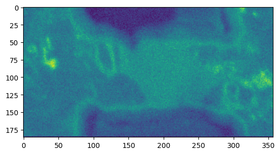
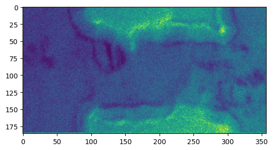
Let’s plot the stddev of each frame:

plt.figure()
plt.imshow(res_stats['all_stats'].data[..., 3])

<matplotlib.image.AxesImage at 0x7f4a1e4fca00>

kind=”sig” buffers, merge functions

• Previously: one result for each scan position

• Now: result buffer shaped like the diffraction patterns

• We need a merge function to merge the result of one partition into the final result

• Different buffer kinds can be combined in a single UDF, so you can combine different operations in a single pass over the data

class MaxFrameUDF(UDF):
    def get_result_buffers(self):
        return {
            'maxframe': self.buffer(kind='sig', dtype='float32')
        }

    def process_frame(self, frame):
        # element-wise maximum:
        self.results.maxframe[:] = np.maximum(self.results.maxframe, frame)

    def merge(self, dest, src):
        # src: the maximum observed in the current partition
        # dest: the maximum observed in all partitions that were already merged together
        dest.maxframe[:] = np.maximum(dest.maxframe, src.maxframe)

res_max = ctx.run_udf(dataset=ds, udf=MaxFrameUDF(), progress=True)

plt.figure()
plt.imshow(np.log1p(res_max['maxframe']))

<matplotlib.image.AxesImage at 0x7f4a2ed1a710>

Region of interest

• work on a subset of the navigation axes

• can be used with all UDFs

• useful for working selectively on data, or just reducing the I/O and computational load when implementing a new UDF

• defined as a binary mask

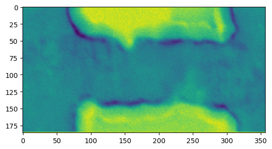
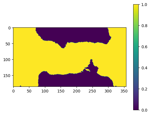
Let’s create a mask based on the previously calculated pixel-sum:

from skimage.morphology import opening, closing

np.min(res_pixelsum_1),  np.max(res_pixelsum_1), np.mean(res_pixelsum_1)

(7762.0, 12367.0, 10277.385)

mask = res_pixelsum_1.data < np.mean(res_pixelsum_1)
# mask = opening(mask)
mask = closing(opening(mask))

plt.figure()
plt.imshow(mask.astype("float32"))
plt.colorbar()

<matplotlib.colorbar.Colorbar at 0x7f4a1d36f100>

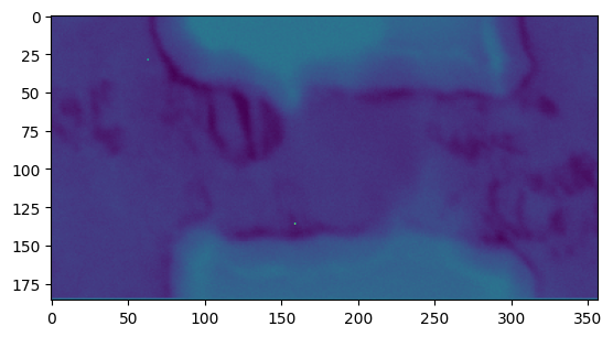
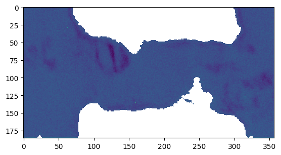
res_roi = ctx.run_udf(dataset=ds, udf=StatsUDF(), roi=mask, progress=True)

plt.figure()
plt.imshow(np.log1p(res_roi['all_stats'].data[..., 2]))

<matplotlib.image.AxesImage at 0x7f4a1cf91c90>

Results with ROI applied

One has to take some care when handling results where a roi was applied; just using the result as a numpy array or accessing the data attribute will give you a result that keeps the whole dataset shape, where the deselected parts are filled with NaN values:

res_roi['all_stats'].data.shape

(186, 357, 4)

There is a second attribute, raw_data, which will give you a flattenned array of just the results, like numpy would give you for fancy indexing:

res_roi['all_stats'].raw_data.shape

(45358, 4)

Parameters

Keyword arguments passed to the UDF are made available in self.params on the UDF. A good convention to document your parameters is to put a docstring into your __init__ method and just pass on the values to super().__init__. You can also validate the arguments here.

class PixelPicker(UDF):
    def __init__(self, coords, *args, **kwargs):
        """
        Parameters
        ----------
        coords : Tuple[int]
            The coordinates to look at in each frame
        """
        if len(coords) != 2:
            raise ValueError("invalid coordinates")
        super().__init__(*args, coords=coords, **kwargs)

    def get_result_buffers(self):
        return {
            'value_of_pixel': self.buffer(kind='nav', dtype=np.float32)
        }

    def process_frame(self, frame):
        self.results.value_of_pixel[:] = frame[self.params.coords]

res_pixel_picker = ctx.run_udf(dataset=ds, udf=PixelPicker(coords=(128, 128)), progress=True)

plt.figure()
plt.imshow(res_pixel_picker['value_of_pixel'])

<matplotlib.image.AxesImage at 0x7f4a1cdf1ed0>