Alignment of phase images
The notebook loads holography reconstruction results from a sample of a iron oxide nanoparticle using magnetization reversal to remove the mean inner potential (MIP), which leaves us with the magnetic phase.
Note
This notebook demonstrates an optional GUI component, among other things, which needs additional dependencies. These can be installed using, for example: pip install libertem-holo[gui].
Packages
[1]:
from IPython import get_ipython
from pathlib import Path
import os
testdata_base_path = os.environ.get("TESTDATA_BASE_PATH")
if testdata_base_path is not None:
    testdata_base_path = Path(testdata_base_path)
[2]:
# Matplotlib widget magic
if os.environ.get("GENERATING_NOTEBOOKS"):
    get_ipython().run_line_magic("matplotlib", "inline")
else:
    get_ipython().run_line_magic("matplotlib", "widget")
[3]:
import matplotlib.pyplot as plt
import numpy as np
from tqdm.notebook import tqdm
from scipy.ndimage import shift
from skimage.transform import warp
from scipy.ndimage import sobel, gaussian_filter
[4]:
from libertem_holo.base.io import Results
from libertem_holo.base.align import ImageCorrelator
from libertem_holo.base.fine_adjust import fine_adjust
from libertem_holo.base.filters import clipped
from libertem_holo.base.unwrap import phase_unwrap, quality_unwrap, derivative_variance
Prepare input data
Before continuing, download the files called minus.npz and plus.npz from https://zenodo.org/uploads/21108532 and put it into the same folder as this notebook. For example using wget:
wget -O minus.npz 'https://zenodo.org/records/21108532/files/minus.npz?download=1'

wget -O plus.npz 'https://zenodo.org/records/21108532/files/plus.npz?download=1'
[5]:
# only for our internal testing:
if testdata_base_path is not None:
    minus_path = testdata_base_path / "dm/holo/align/minus.npz"
    plus_path = testdata_base_path / "dm/holo/align/plus.npz"
else:
    minus_path = Path(".") / "minus.npz"
    plus_path = Path(".") / "plus.npz"
Load data
Data is loaded directly as a Results object from the previous reconstruction notebook. The dataset contains the complex wave, the unwrapped phase, the brightfield image as well as some metadata information (like pixel size).
[6]:
data_minus = Results.load(minus_path)
data_plus = Results.load(plus_path)
In this example notebook, two stacks of holograms were acquired on the same Fe3O4 nanoparticle after excitation from the objective lens in two different magnetic field: +1 T (data_plus) and -1 T (data_minus). The magnetization is reversed between both datasets, allowing the substraction of Mean Inner Potential (MIP). The alignment of both phase images will be described using 2 differents methods: phase cross correlation and manual alignment using an interactive GUI.
[7]:
fig, ax = plt.subplots(ncols=2, figsize=(12, 6))
ax[0].imshow(data_minus.unwrapped_phase)
ax[0].axis('off')
ax[0].set_title('Unwrapped phase of Minus dataset')
ax[1].imshow(data_plus.unwrapped_phase)
ax[1].axis('off')
ax[1].set_title('Unwrapped phase of Plus dataset')
[7]:
Text(0.5, 1.0, 'Unwrapped phase of Plus dataset')
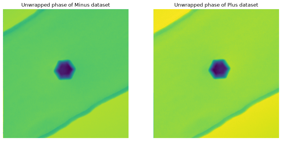
The phase or the brightfield can be used for alignment. The advantage of the brightfield image is to not possess any artefacts from magnetization or electrostatic potential difference between datasets.
[8]:
phase_minus = data_minus.unwrapped_phase
phase_plus = data_plus.unwrapped_phase
[9]:
bf_minus = data_minus.brightfield
bf_plus = data_plus.brightfield
Cross correlation
A common method for image alignment is cross correlation. The cross correlation class can be used with different types of parameters, but the outline remains the same:
Initialize the
ImageCorrelatorobjectPrepare the inputs
Correlate the inputs
Shift the moving input based on the maximum of the correlation map
The Correlator determines how the images are pre-filtered, and how the correlation map is constructed in detail.
[10]:
correlator = ImageCorrelator(
    hanning=True,  # without hanning filter, correlation might have cross artifacts becuase of edge effects
    binning=2,  # helps against misalignment caused by noise, can also improve performance
    upsample_factor=10,  # enable subpixel precision
    normalization='phase',  # use phase cross correlation. Set to `None` on very noisy data
    xp=np,  # set to `cupy` for GPU-accelerated filtering and correlation
)
Region of interest is selected around the particle to only align object features, and ignore any potential artifacts at the edges:
[11]:
roi = np.s_[100:-100, 100:-100]
[12]:
ref_image = correlator.prepare_input(bf_minus[roi])
moving_image = correlator.prepare_input(bf_plus[roi])
[13]:
corr_results = correlator.correlate(ref_image, moving_image)
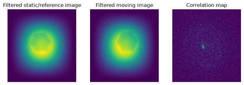
The correlation map can be plotted to check the spread of the maximum, or potential artefacts from the FFTs.
[14]:
fig, ax = plt.subplots(ncols=3, figsize=(10,5))
ax[0].imshow(np.abs(ref_image))
ax[0].set_title('Filtered static/reference image')
ax[0].axis("off")
ax[1].imshow(np.abs(moving_image))
ax[1].set_title('Filtered moving image')
ax[1].axis("off")
ax[2].imshow(corr_results.corrmap)
ax[2].set_title('Correlation map')
ax[2].axis("off")
[14]:
(np.float64(-0.5), np.float64(131.5), np.float64(139.5), np.float64(-0.5))
[15]:
corr_results.shift
[15]:
(np.float64(2.5999999999999943), np.float64(-15.200000000000003))
[16]:
phase_plus_shifted = shift(phase_plus, corr_results.shift)
[17]:
fig, ax = plt.subplots(ncols=3, figsize=(10, 5), sharex=True, sharey=True)
ax[0].imshow(phase_minus)
ax[0].set_title('Original static phase')
ax[1].imshow(phase_plus_shifted)
ax[1].set_title('Shifted moving phase')
ax[2].imshow(phase_minus - phase_plus_shifted)
ax[2].set_title('Difference of phases from alignment')
[17]:
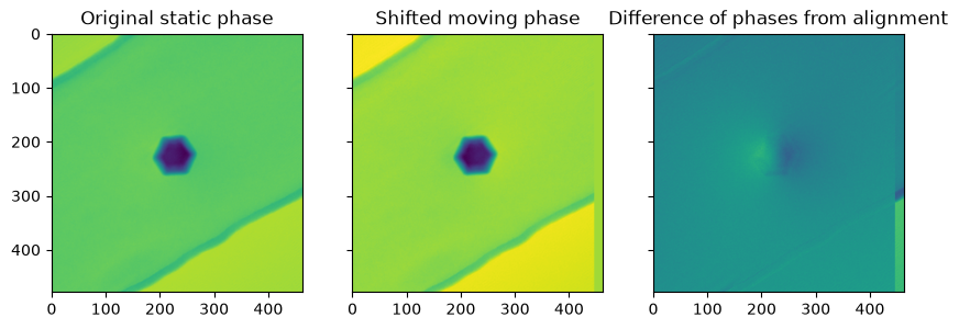
Text(0.5, 1.0, 'Difference of phases from alignment')
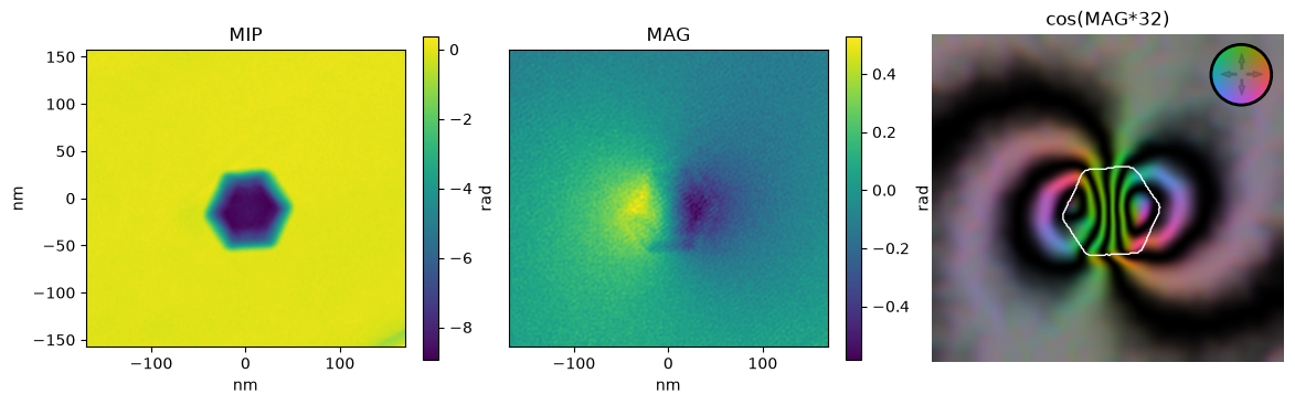
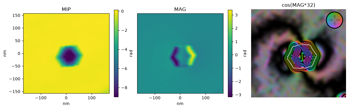
MIP and magnetic phase can now be calculated.
[18]:
MIP_phase = (phase_minus + phase_plus_shifted) / 2
MIP_phase -= np.mean(MIP_phase)
MAG_phase = (phase_minus - phase_plus_shifted) / 2
MAG_phase -= np.mean(MAG_phase)
For induction field lines visualisation, a cosine can be applied to the magnetic phase. A convenient function can be imported.
[19]:
from libertem_holo.base.convenience import plot_mag_induction
[20]:
# the phase images can be cropped to remove the drift corrected edges
# and use calibrated units for the axis in nm
roi = np.s_[80:350, 80:370]
extent = (
    -MIP_phase[roi].shape[1] * data_minus.metadata['effective_pixelsize']/2 * 1e9,
    MIP_phase[roi].shape[1] * data_minus.metadata['effective_pixelsize']/2 * 1e9,
    -MIP_phase[roi].shape[0] * data_minus.metadata['effective_pixelsize']/2 * 1e9,
    MIP_phase[roi].shape[0] * data_minus.metadata['effective_pixelsize']/2 * 1e9,
)
[21]:
fig, ax = plt.subplots(ncols=3, figsize=(14, 6))

im = ax[0].imshow(MIP_phase[roi], extent=extent)
ax[0].set_title('MIP')
ax[0].set_xlabel('nm')
ax[0].set_ylabel('nm')
plt.colorbar(im, fraction=0.046, label='rad')

im = ax[1].imshow(MAG_phase[roi], extent=extent)
ax[1].set_title('MAG')
ax[1].set_xlabel('nm')
ax[1].set_yticks([])
plt.colorbar(im, fraction=0.046, label='rad')

mask = MIP_phase[roi] < -1.5
ax[2] = plot_mag_induction(MAG_phase[roi], axis=ax[2], clip=1e-2, gain=32, smooth=5, mask=mask)
ax[2].set_title('cos(MAG*32)')
ax[2].axis('off')
[21]:
(np.float64(0.0), np.float64(290.0), np.float64(0.0), np.float64(270.0))
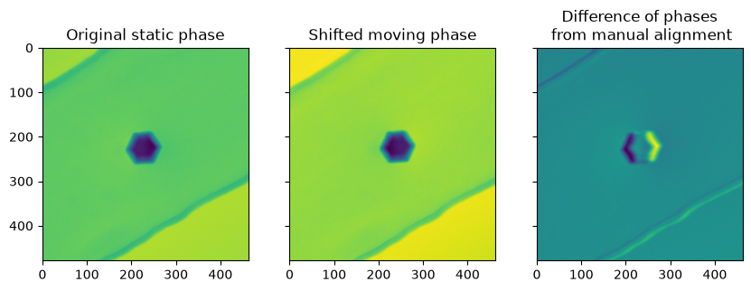
Manual alignment
If the cross correlation is not working (data too noisy) or if there is both translation and rotation transformation, a manual alignment can be necessary. This section depends on interactive feedback from the user, so it works best if used in jupyterlab.
[22]:
fig, getter = fine_adjust(static=phase_minus, moving=phase_plus)
fig
[22]:
[23]:
transf_matrix = getter()
[24]:
phase_plus_shifted = warp(phase_plus, transf_matrix)
[25]:
fig, ax = plt.subplots(ncols=3, figsize=(10, 5), sharex=True, sharey=True)
ax[0].imshow(phase_minus)
ax[0].set_title('Original static phase')
ax[1].imshow(phase_plus_shifted)
ax[1].set_title('Shifted moving phase')
ax[2].imshow(phase_minus - phase_plus_shifted)
ax[2].set_title('Difference of phases\n from manual alignment')
[25]:
Text(0.5, 1.0, 'Difference of phases\n from manual alignment')
[26]:
MIP_phase = (phase_minus + phase_plus_shifted) / 2
MIP_phase -= np.mean(MIP_phase)
MAG_phase = (phase_minus - phase_plus_shifted) / 2
MAG_phase -= np.mean(MAG_phase)
[27]:
roi = np.s_[80:350, 80:370]
extent = (
    -MIP_phase[roi].shape[1] * data_minus.metadata['effective_pixelsize']/2 * 1e9,
    MIP_phase[roi].shape[1] * data_minus.metadata['effective_pixelsize']/2 * 1e9,
    -MIP_phase[roi].shape[0] * data_minus.metadata['effective_pixelsize']/2 * 1e9,
    MIP_phase[roi].shape[0] * data_minus.metadata['effective_pixelsize']/2 * 1e9,
)
[28]:
fig, ax = plt.subplots(ncols=3, figsize=(14, 6))

im = ax[0].imshow(MIP_phase[roi], extent=extent)
ax[0].set_title('MIP')
ax[0].set_xlabel('nm')
ax[0].set_ylabel('nm')
plt.colorbar(im, fraction=0.046, label='rad')

im = ax[1].imshow(MAG_phase[roi], extent=extent)
ax[1].set_title('MAG')
ax[1].set_xlabel('nm')
ax[1].set_yticks([])
plt.colorbar(im, fraction=0.046, label='rad')

mask = MIP_phase[roi] < -1.5
ax[2] = plot_mag_induction(MAG_phase[roi], axis=ax[2], clip=1e-2, gain=32, smooth=5, mask=mask)
ax[2].set_title('cos(MAG*32)')
ax[2].axis('off')
[28]:
(np.float64(0.0), np.float64(290.0), np.float64(0.0), np.float64(270.0))
[ ]: