Upsampling-based subpixel refinement

This notebook demonstrates the use of DFT-upsampling-based subpixel refinement when running blobfinder, which gives more precise results than the standard approach at the expense of computation time.

%matplotlib inline

import numpy as np
import matplotlib.pyplot as plt
import libertem.api as lt
from scipy.ndimage import fourier_shift

from libertem_blobfinder.base.utils import cbed_frame
from libertem_blobfinder.common.patterns import Circular
from libertem_blobfinder.udf.correlation import run_blobfinder

Dataset

We generate a small, demo dataset containing a single circular disk which is shifted by a small amount across ecah frame in the scan grid:

nav_shape = (12, 45)
sig_shape = (64, 64)
radius = 6
ny, nx = nav_shape
yshift = (-1, 1)  # px
xshift = (-3, 3)  # px

The image shifting is performed using the Fourier method to give a result independent of the pixel grid:

frame, _, _ = cbed_frame(*sig_shape, radius=radius, a=(100, 100), b=(100, 100))
frame = frame[0]
frame_fft = np.fft.fft2(frame.astype(np.float32))
frames = np.zeros(nav_shape + sig_shape, dtype=np.float32)
true_shifts = np.zeros(nav_shape + (2,))
for yi, yd in enumerate(np.linspace(*yshift, num=ny, endpoint=True)):
    for xi, xd in enumerate(np.linspace(*xshift, num=nx, endpoint=True)):
        true_shifts[yi, xi] = (yd * (-1 * xi / nx), xd * (yi / ny))
        frames[yi, xi, ...] = np.fft.ifft2(
            fourier_shift(frame_fft, true_shifts[yi, xi])
        ).real.astype(np.float32)

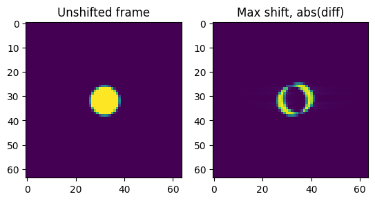
The maximum shift in the dataset is on the order of 3 px.

fig, (ax1, ax2) = plt.subplots(1, 2)
ax1.imshow(frame)
ax1.set_title('Unshifted frame')
ax2.imshow(np.abs(frame - frames[-1, -1]))
ax2.set_title('Max shift, abs(diff)');

Run blobfinder

The dataset is small so we will use an inline Context and a dataset in memory.

ctx = lt.Context.make_with('inline')
ds = ctx.load('memory', data=frames)

Without upsampling

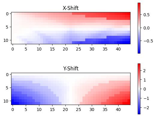
By default blobfinder calculates subpixel peak positions using a local centre-of-mass around the maxima of the correlation map.

sum_result, centers, refineds, peak_values, peak_elevations, peaks = run_blobfinder(
    ctx,
    ds,
    match_pattern=Circular(radius),
    num_peaks=1,
    upsample=False,
)

This approach leads to aliasing on the order of +/- 0.3 px. This becomes visible when the maximium shifts in a dataset are small. The aliasing is visible as banding in the color plot for each dimension:

fig, (ax1, ax2) = plt.subplots(2, 1)
shifts = (refineds.data - np.asarray(sig_shape) // 2)[..., 0, :]
im = ax1.imshow(shifts[..., 0], cmap='bwr')
ax1.set_title('X-Shift')
plt.colorbar(im, ax=ax1)
im = ax2.imshow(shifts[..., 1], cmap='bwr')
ax2.set_title('Y-Shift')
plt.colorbar(im, ax=ax2);

With upsampling

Using the upsample=True option on any of the blobfinder API endpoints enables sub-pixel precision calculated using upsampling of the DFT of the correlation map, rather than centre-of-mass. This increases the computation time but can be worth it to remove aliasing.

By default an upsampling of 20x is used but the argument also accepts an integer to specify more or less precision.

sum_result, centers, refineds, peak_values, peak_elevations, peaks = run_blobfinder(
    ctx,
    ds,
    match_pattern=Circular(radius),
    num_peaks=1,
    upsample=True,
)

It is clear from the lack of color banding that the aliasing is reduced in this case.

fig, (ax1, ax2) = plt.subplots(2, 1)
shifts_us = (refineds.data - np.asarray(sig_shape) // 2)[..., 0, :]
im = ax1.imshow(shifts_us[..., 0], cmap='bwr')
ax1.set_title('X-Shift')
plt.colorbar(im, ax=ax1)
im = ax2.imshow(shifts_us[..., 1], cmap='bwr')
ax2.set_title('Y-Shift')
plt.colorbar(im, ax=ax2);

Comparison

As we have only a single disk in the frame we can measure the shift using CoM directly:

cy, cx = np.asarray(sig_shape) // 2
com_a = ctx.create_com_analysis(ds, cx=cx, cy=cy)
com_r = ctx.run(com_a)
y_shift_com = com_r.y.raw_data

We see that the frame CoM result precisely matches the shifts used when generating the dataset.

fig, ax = plt.subplots()
sl = np.s_[9, :, 0]
xvals = np.arange(true_shifts[sl].size)
ax.plot(xvals, true_shifts[sl], 'k', label="True shift", linewidth=2)
ax.plot(xvals, y_shift_com[sl[:2]], 'g--', label="Frame CoM")
ax.plot(xvals, shifts[sl], 'r', label="CoM refinement")
ax.plot(xvals, shifts_us[sl], 'b', label="Upsampling refinement")
ax.set_xlabel('Scan x-coordinate')
ax.set_ylabel('Peak y-shift')
ax.set_title(f'y-shifts for row {sl[0]}')
ax.legend();

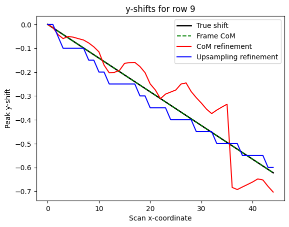
In addition, we see the strong aliasing in the standard CoM-based refinement, and the reduced aliasing when using upsampling. The steps in the upsampling curve are due to the default upsampling factor of 20x, which means the precision of the subpixel centre is at most 1 /  20 == 0.05 px. This can be improved by passing the desired upsampling factor to the blobfinder api.

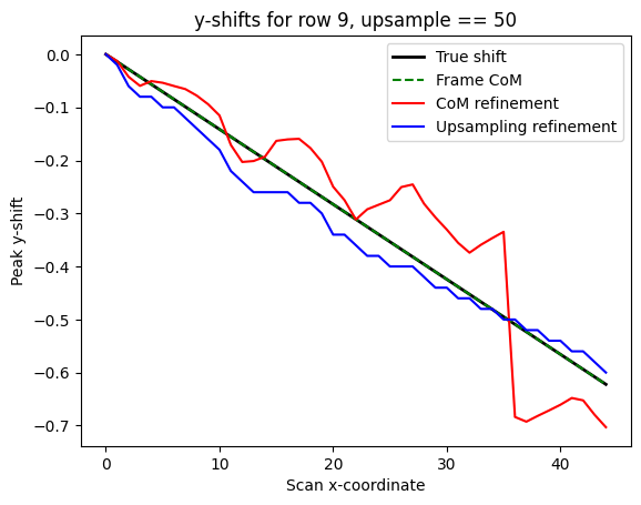
With upsample == 50

upsample_f = 50
sum_result, centers, refineds, peak_values, peak_elevations, peaks = run_blobfinder(
    ctx,
    ds,
    match_pattern=Circular(radius),
    num_peaks=1,
    upsample=upsample_f,
)
shifts_us50 = (refineds.data - np.asarray(sig_shape) // 2)[..., 0, :]

fig, ax = plt.subplots()
xvals = np.arange(true_shifts[sl].size)
ax.plot(xvals, true_shifts[sl], 'k', label="True shift", linewidth=2)
ax.plot(xvals, y_shift_com[sl[:2]], 'g--', label="Frame CoM")
ax.plot(xvals, shifts[sl], 'r', label="CoM refinement")
ax.plot(xvals, shifts_us50[sl], 'b', label="Upsampling refinement")
ax.set_xlabel('Scan x-coordinate')
ax.set_ylabel('Peak y-shift')
ax.set_title(f'y-shifts for row {sl[0]}, upsample == {upsample_f}')
ax.legend();